3 Real Numbers
In this chapter we introduce the system of Real Numbers \(\mathbb{R}\) and study some of its properties. We will follow quite an abstract approach, which requires the definition of ordered field. The fact that \(\mathbb{R}\) is a continuum with no gaps (unlike \(\mathbb{Q}\)) will be consequence of the Axiom of Completeness.
Therefore \(\mathbb{R}\) will be defined as an ordered field in which the Axiom of Completeness holds.
3.1 Fields
In order to introduce \(\mathbb{R}\), we need the concepts of binary operation and field. We proceed in a general setting, starting from a set \(K\). We will assume that there is an equivalence relation on \(K\) denoted by \(=\).
Definition 1: Binary operation
Notation 2
We use the special symbols of \(+\) and \(\cdot\) to refer to addition and multiplication.
- Addition: The addition, or sum of \(x,y \in K\) is denoted by \[ x + y \]
- Multiplication: The multiplication, or product of \(x,y \in K\) is denoted by \[ x \cdot y \,\, \mbox{ or } \,\, xy \]
Warning
Example 3: An example of binary operation
Note that we have defined (rather controversially!) \[ 1+1 = 0 \] The other option would have been to define \[ 1 + 1 = 1 \] This would have been absolutely fine. However we could not have defined \[ 1 + 1 = 2 \] because \(2 \notin K\).
Note: The operations in (3.1) look more natural if you identify \(0\) with the even numbers and \(1\) with the odd numbers. In that case \(1+1 = 0\) reads \[ \mathrm{Odd} + \mathrm{Odd} = \mathrm{Even} \] Indeed all the definitions given in (3.1) agree with such identification, see tables below: \[ \begin{array}{c|cc} + & \mathrm{Even} & \mathrm{Odd} \\ \hline \mathrm{Even} & \mathrm{Even} & \mathrm{Odd} \\ \mathrm{Odd} & \mathrm{Odd} & \mathrm{Even} \\ \end{array} \qquad \qquad \begin{array}{c|cc} \cdot & \mathrm{Even} & \mathrm{Odd} \\ \hline \mathrm{Even} & \mathrm{Even} & \mathrm{Even} \\ \mathrm{Odd} & \mathrm{Even} & \mathrm{Odd} \\ \end{array} \]
Binary operations take ordered pairs of elements of \(K\) as input. Therefore the operation \[ x \circ y \circ z \] does not make sense, since we do not know which one between \[ x \circ y \quad \mbox{ or } \quad y \circ z \] has to be performed first. Moreover the outcome of an operation depends on order: \[ x \circ y \neq y \circ x \,. \] This motivates the following definition.
Definition 4: Properties of binary operations
Let \(K\) be a set and \(\circ \ \colon K \times K \to K\) be a binary operation on \(K\). We say that:
- \(\circ\) is commutative if \[ x \circ y = y \circ x \,, \quad \, \forall \, x,y \in K \]
- \(\circ\) is associative if \[ (x \circ y) \circ z = x \circ (y \circ z) \,, \quad \, \forall \, x,y,z \in K \]
- An element \(e \in K\) is called neutral element of \(\circ\) if \[ x \circ e = e \circ x = x \,, \quad \, \forall \, x \in K \]
- Let \(e\) be a neutral element of \(\circ\) and let \(x \in K\). An element \(y \in K\) is called an inverse of \(x\) with respect to \(\circ\) if \[ x \circ y = y \circ x = e \,. \]
Example 5
Consider \(\mathbb{Q}\) with the usual operations of sum and multiplication
We already know that \(+\) and \(\cdot\) are commutative and associative
The neutral element of the sum is \(e = 0\)
The neutral element of the product is \(e = 1\)
The additive inverse of \(x\) is \(-x\)
The multiplicative inverse of \(x \neq 0\) is \(1/x\).
Example 6
Let \(K\) with \(+\) and \(\cdot\) be as in Example 3. The sum satisfies:
- \(+\) is commutative, since \[ 0 + 1 = 1 + 0 = 0 \,. \]
- \(+\) is associative, since for example \[ (0 + 1) + 1 = 1 + 1 = 0 \,, \quad 0 + (1 + 1) = 0 + 0 = 0 \,, \] and therefore \[ (0 + 1) + 1 = 0 + (1 + 1) \,. \] In general one can show that \(+\) is associative by checking all the other permutations.
- The neutral element of \(+\) is \(0\), since \[ 0 + 0 = 0 \,, \quad 1 + 0 = 0 + 1 = 1 \,. \]
- Every element has an inverse. Indeed, the inverse of \(0\) is \(0\), since \[ 0 + 0 = 0\,, \] while the inverse of \(1\) is \(1\), since \[ 1 + 1 = 1 + 1 = 0 \,. \]
The multiplication satisfies:
- \(\cdot\) is commutative, since \[ 1 \cdot 0 = 0 \cdot 1 = 0 \,. \]
- \(\cdot\) is associative, since for example \[ (0 \cdot 1) \cdot 1 = 0 \cdot 1 = 0 \,, \quad 0 \cdot (1 \cdot 1) = 0 \cdot 1 = 0 \,, \] and therefore \[ (0 \cdot 1) \cdot 1 = 0 \cdot (1 \cdot 1) \,. \] By checking all the other permutations one can show that \(\cdot\) is associative.
- The neutral element of \(\cdot\) is \(1\), since \[ 0 \cdot 1 = 1 \cdot 0 = 0 \,, \quad 1 \cdot 1 = 1 \,. \]
- The element \(0\) has no inverse, since
\[ 0 \cdot 0 = 0 \cdot 1 = 1 \cdot 0 = 0\,, \] and thus we never obtain the neutral element \(1\). The inverse of \(1\) is given by \(1\), since \[ 1 \cdot 1 = 1 \,. \]
Example 7
Question. Let \(K=\{0,1\}\) be a set with binary operation \(\circ\) defined by the table \[ \begin{array}{c|cc} \circ & 0 & 1 \\ \hline 0 & 1 & 1 \\ 1 & 0 & 0 \\ \end{array} \]
Is \(\circ\) commutative? Justify your answer.
Is \(\circ\) associative? Justify your answer.
Solution.
The operation \(\circ\) is not commutative, since \[ 0 \circ 1 = 1 \neq 0 = 1 \circ 0 \,. \]
The operation \(\circ\) is not associative, since \[ (0 \circ 1) \circ 1 = 1 \circ 1 = 0 \,, \] while \[ 0 \circ (1 \circ 1) = 0 \circ 0 = 1 \,, \] so that \[ (0 \circ 1) \circ 1 \neq 0 \circ (1 \circ 1)\,. \]
We are ready to define fields.
Definition 8: Field
Let \(K\) be a set with binary operations of addition \[ +\ \colon K \times K \to K \,, \quad (x,y) \mapsto x + y \] and multiplication \[ \cdot\ \colon K \times K \to K \,, \quad (x,y) \mapsto x \cdot y = xy \,. \] We call the triple \((K, + , \cdot)\) a field if:
- The addition \(+\) satisfies: \(\,\forall \, x,y,z \in K\)
- (A1) Commutativity and Associativity: \[ x+y = y+x \] \[ (x+y)+z = x+(y+z) \]
- (A2) Additive Identity: There exists a neutral element in \(K\) for \(+\), which we call \(0\). It holds: \[ x + 0 = 0 + x = x \]
- (A3) Additive Inverse: There exists an inverse of \(x\) with respect to \(+\). We call this element the additive inverse of \(x\) and denote it by \(-x\). It holds \[ x + (-x) = (-x) + x = 0 \]
- The multiplication \(\cdot\) satisifes: \(\,\forall \, x,y,z \in K\)
- (M1) Commutativity and Associativity: \[ x \cdot y = y \cdot x \] \[ (x \cdot y) \cdot z = x \cdot (y \cdot z) \]
- (M2) Multiplicative Identity: There exists a neutral element in \(K\) for \(\cdot\), which we call \(1\). It holds: \[ x \cdot 1 = 1 \cdot x = x \]
- (M3) Multiplicative Inverse: If \(x \neq 0\) there exists an inverse of \(x\) with respect to \(\cdot\). We call this element the multiplicative inverse of \(x\) and denote it by \(x^{-1}\). It holds \[ x \cdot x^{-1} = x^{-1} \cdot x = 1 \]
- The operations \(+\) and \(\cdot\) are related by
- (AM) Distributive Property: \(\,\forall \, x,y,z \in K\) \[ x \cdot (y + z) = (x \cdot y) + (y \cdot z) \,. \]
Remark 9
Warning
Example 10
Question. Let \(K\) with \(+\) and \(\cdot\) be as in Example 3, that is, \(K=\{0,1\}\) with operations defined by \[ \begin{array}{c|cc} + & 0 & 1 \\ \hline 0 & 0 & 1 \\ 1 & 1 & 0 \\ \end{array} \qquad \qquad \begin{array}{c|cc} \cdot & 0 & 1 \\ \hline 0 & 0 & 0 \\ 1 & 0 & 1 \\ \end{array} \] Prove that \((K,+,\cdot)\) is a field.
Solution. We have already shown in Example 6 that:
- (A1) and (M1) hold,
- (A2) holds with neutral element \(0\),
- (M2) holds with neutral element \(1\),
- (A3) every element has an additive inverse, with \[ -0 = 0 \,, \quad - 1 = 1 \,, \]
- (M3) every element which is not \(0\) a multiplicative inverse, with \[ 1^{-1} = 1\,. \]
We are left to show the Distributive Property (AM). Indeed:
- (AM) For all \(y,z \in K\) we have \[ 0 \cdot (y + z) = 0 \,, \quad (0 \cdot y) + (0 \cdot z) = 0 + 0 = 0\,, \] and also \[ 1 \cdot (y + z) = y + z \,, \quad (1 \cdot y) + (1 \cdot z) = y + z \,. \] Thus (AM) holds.
Definition 11: Subtraction and division
Let \((K,+,\cdot)\) be a field. We define:
Subtraction as the operation \(-\) defined by \[ x - y := x + (-y) \,, \quad \forall \, x , y \in K \,, \] where \(-y\) is the additive inverse of \(y\).
Division as the operation \(/\) defined by \[ x/y := x \cdot y^{-1}\,, \quad \forall \, x , y \in K \,, \,\, y \neq 0 \,, \] where \(y^{-1}\) is the multiplicative inverse of \(y\).
Warning
Using the field axioms we can prove the following properties.
Proposition 12: Uniqueness of neutral elements and inverses
Let \((K,+,\cdot)\) be a field. Then
- There is a unique element in \(K\) with the property of \(0\),
- There is a unique element in \(K\) with the property of \(1\),
- For all \(x \in K\) there is a unique additive inverse \(-x\),
- For all \(x \in K\), \(x \neq 0\), there is a unique multiplicative inverse \(x^{-1}\).
Proof
- Suppose that \(0 \in K\) and \(\widetilde{0} \in K\) are both neutral element of \(+\), that is, they both satisfy (A2). Then \[ 0 + \widetilde{0} = 0 \] since \(\widetilde{0}\) is a neutral element for \(+\). Moreover \[ \widetilde{0} + 0 = \widetilde{0} \] since \(0\) is a neutral element for \(+\). By commutativity of \(+\), see property (A1), we have \[ 0 = 0 + \widetilde{0} = \widetilde{0} + 0 = \widetilde{0} \,, \] showing that \(0 = \widetilde{0}\). Hence the neutral element for \(+\) is unique.
- Exercise.
- Let \(x \in K\) and suppose that \(y, \widetilde{y} \in K\) are both additive inverses of \(x\), that is, they both satisfy (A3). Therefore \[ x + y = 0 \] since \(y\) is an additive inverse of \(x\) and \[ x + \widetilde{y} = 0 \] since \(\widetilde{y}\) is an additive inverse of \(x\). Therefore we can use commutativity and associativity and of \(+\), see property (A1), and the fact that \(0\) is the neutral element of \(+\), to infer \[\begin{align*} y & = y + 0 = y + (x + \widetilde{y}) \\ & = (y + x) + \widetilde{y} = (x + y) + \widetilde{y} \\ & = 0 + \widetilde{y} = \widetilde{y} \,, \end{align*}\] concluding that \(y = \widetilde{y}\). Thus there is a unique additive inverse of \(x\), and \[ y = \widetilde{y} = -x \,, \] with \(-x\) the element from property (A3).
- Exercise.
Using the properties of field we can also show that the usual properties of sum, subtraction, multiplication and division still hold in any field. We list such properties in the following proposition.
Proposition 13: Properties of field operations
Let \((K,+,\cdot)\) be a field. Then for all \(x,y,z \in K\),
- \(x + y = x + z \,\, \implies \,\, y = z\)
- \(x \cdot y = x \cdot z \,\) and \(\,x \neq 0 \,\, \implies \,\, y = z\)
- \(- 0 = 0\)
- \(1^{-1} = 1\)
- \(x \cdot 0 = 0\)
- \(-1 \cdot x = -x\)
- \(-(-x) = x\)
- \((x^{-1})^{-1} = x \,\) if \(\, x \neq 0\)
- \((x \cdot y)^{-1} = x^{-1} \cdot y^{-1}\)
The above properties can be all proven with elementary use of the field properties (A1)-(A3), (M1)-(M3) and (AM). This is an exercise in patience, and is left to the reader.
Let us conclude with examining the sets of numbers introduced in Chapter 1.
Theorem 14
Consider the sets \(\mathbb{N}\), \(\mathbb{Z}\), \(\mathbb{Q}\) with the usual operations \(+\) and \(\cdot\). We have:
\((\mathbb{N}, + , \cdot)\) is not a field.
\((\mathbb{Z}, + , \cdot)\) is not a field.
\((\mathbb{Q}, + , \cdot)\) is a field.
Proof
- \((\mathbb{N}, + , \cdot)\) is not a field:
It satisfies properties (A1), (A2), (M1), (M2), (AM) of fields. It is missing properties (A3) and (M3), the additive and multiplicative inverse properties, respectively.
\((\mathbb{Z}, + , \cdot)\) is not a field:
It satisfies properties (A1), (A2), (A3), (M1), (M2), (AM) of fields. Thus it is only missing (M3), the multiplicative inverse property.\((\mathbb{Q}, + , \cdot)\) is a field. This is clear: The field axioms are introduced exactly to model \(\mathbb{Q}\). Therefore, \(\mathbb{Q}\) is trivially a field.
3.2 Ordered fields
Definition 15: Ordered field
Let \(K\) be a set with binary operations \(+\) and \(\cdot\), and with an order relation \(\leq\). We call \((K,+,\cdot,\leq)\) an ordered field if:
\((K,+,\cdot)\) is a field
There \(\leq\) is of total order on \(K\): \(\, \forall \, x, y, z \in K\)
- (O1) Reflexivity: \[ x \leq x \]
- (O2) Antisymmetry: \[ x \leq y \, \mbox{ and } \, y \leq x \,\, \implies \,\, x = y \]
- (O3) Transitivity: \[ x \leq y \,\, \mbox{ and } \,\, y \leq z \,\, \implies \,\, x = z \]
- (O4) Total order:
\[ x \leq y \,\, \mbox{ or } \,\, y \leq x \]
The operations \(+\) and \(\cdot\), and the total order \(\leq\), are related by the following properties: \(\, \forall x, y, z \in K\)
- (AM) Distributive: Relates addition and multiplication via \[ x \cdot (y + z) = x \cdot y + x \cdot z \]
- (AO) Relates addition and order with the requirement: \[ x \leq y \,\, \implies \,\, x + z \leq y + z \]
- (MO) Relates multiplication and order with the requirement: \[ x \geq 0, \, y \geq 0 \,\, \implies \,\, x \cdot y \geq 0 \]
Theorem 16
3.3 Cut Property
We have just introduced the notion of fields and ordered fields. We noted that the set of rational numbers with the usual operations of sum and multiplication \[ (\mathbb{Q}, + , \cdot) \] is a field. Moreover it is an ordered field with the usual order \(\leq\).
We now need to address the key issue we proved in Chapter 1, namely, the fact that \[ \sqrt{2} \notin \mathbb{Q}\,. \] Intuitively, this means that \(\mathbb{Q}\) has gaps, and cannot be represented as a continuous line. The rigorous definition of lack of gaps needs the concept of cut of a set. This, in turn, needs the concept of partition.
Definition 17: Partition of a set
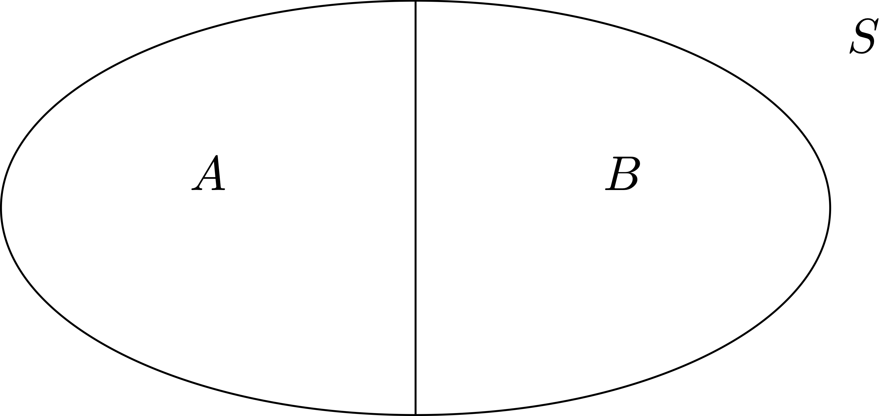
Definition 18: Cut of a set
Let \(S\) be a non-empty set with a total order relation \(\leq\). The pair \((A,B)\) is a cut of \(S\) if
- \((A,B)\) is a partition of \(S\),
- We have \[ a \leq b \,, \quad \forall \, a \in A \,, \,\, \forall \, b \in B \,. \]
The cut of a set is often called Dedekind cut, named after Richard Dedekind, who used cuts to give an explicit construction of the real numbers \(\mathbb{R}\), see Wikipedia page.
Definition 19: Cut property
Example 20
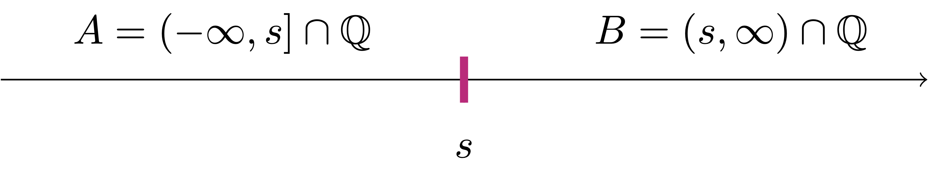
Question 21
The answer to the above question is NO. For example the pair \[ A = (-\infty,\sqrt{2}) \cap \mathbb{Q}\,, \quad B = (\sqrt{2},\infty) \cap \mathbb{Q}\,. \tag{3.2}\] is a cut of \(\mathbb{Q}\), since \(\sqrt{2} \notin \mathbb{Q}\). However what is the separator? It should be \(s = \sqrt{2}\), given that clearly \[ a \leq \sqrt{2} \leq b \,, \quad \forall \, a \in A\,, \,\, \forall \, b \in B \,. \] However \(\sqrt{2} \notin \mathbb{Q}\), so we are NOT ALLOWED to take it as separator. Indeed, we can show that \((A,B)\) defined as in (3.2) has no separator.
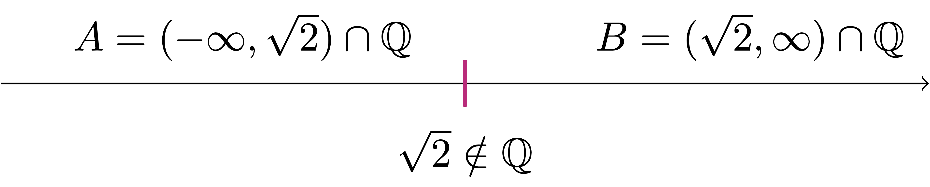
Theorem 22: \(\mathbb{Q}\) does not have the cut property.
Remark 23: Ideas for the proof of Theorem 22
We will consider the cut \((A,B)\) in (3.2). We then assume by contradiction that \((A,B)\) admits a separator \(L \in \mathbb{Q}\), so that \[ a \leq L \leq b \,, \quad \forall \, a \in A\,, \,\, \forall \, b \in B \,. \tag{3.3}\] Since \((A,B)\) is a partition of \(\mathbb{Q}\), then either \(L \in A\) or \(L \in B\). These will both lead to a contradiction:
If \(L \in A\), by definition of \(A\) we have \[ L < \sqrt{2} \,. \] We want to contradict the fact that \(L\) is a separator for the cut \((A,B)\). The idea is that, since \(\sqrt{2} \notin \mathbb{Q}\), it is possible to squeeze a rational number \(\widetilde{L} \in \mathbb{Q}\) in between \(L\) and \(\sqrt{2}\), i.e. \[ L < \widetilde{L} < \sqrt{2} \,. \] How do we find such \(\widetilde{L}\) in practice? We look for a number \(\widetilde{L}_n\) of the form \[ \widetilde{L}_n = L + \frac{1}{n} \] for some \(n \in \mathbb{N}\) to be suitably chosen later. Clearly \(\widetilde{L}_n \in \mathbb{Q}\) and \[ L < \widetilde{L}_n \] for all \(n \in \mathbb{N}\). We will then be able to find \(n_0 \in \mathbb{N}\) such that \[ L < \widetilde{L}_{n_0} < \sqrt{2} \,. \tag{3.4}\] Now comes the contradiction: From (3.4) we see that \(\widetilde{L}_{n_0} \in A\). However \(L\) is a separator, and so from (3.3) we have \[ \widetilde{L}_{n_0} \leq L \,, \] which contradicts (3.4).
If \(L \in B\), by definition of \(B\) we have \[ \sqrt{2} < L \,. \] The idea is the same as above: Since \(\sqrt{2} \notin \mathbb{Q}\), we can squeeze a rational number \(\widetilde{L} \in \mathbb{Q}\) between \(\sqrt{2}\) and \(L\), i.e., \[ \sqrt{2} < \widetilde{L} < L \,. \] Since we want \(\widetilde{L}\) to be a rational number smaller than \(L\), we look for \(\widetilde{L}\) of the form \[ \widetilde{L}_n := L - \frac{1}{n} \,, \] for a suitable \(n \in \mathbb{N}\). Clearly \(\widetilde{L}_n \in \mathbb{Q}\) and \[ \widetilde{L}_n < L \,, \] for all \(n \in \mathbb{N}\). We will be able to find \(n_0 \in \mathbb{N}\) such that \[ \sqrt{2} < \widetilde{L}_{n_0} < L \,. \tag{3.5}\] Therefore \(\widetilde{L}_{n_0} \in B\). Again, contradiction: \(L\) is a separator and so \[ L \leq \widetilde{L}_{n_0} \,, \] which contradicts (3.5).
Both cases \(L \in A\) or \(L \in B\) lead to a contradiction. Since these are all the possibilities, we conclude that the cut \((A,B)\) has no separator in \(\mathbb{Q}\).
Time to make the ideas in the above remark rigorous. Two main issues need fixing:
\(\sqrt{2}\) is just a symbol for a number \(x\) such that \(x^2 = 2\). As \(\sqrt{2} \notin \mathbb{Q}\), what is the meaning of the expression \[ a < \sqrt{2} < b \] when \(a,b \in \mathbb{Q}\)? We can only compare rational numbers with rational numbers, so the above inequalities are meaningless. We need a more clever way to write down the sets \(A\) and \(B\) so that they make sense as objects in \(\mathbb{Q}\).
We said it is possible to find \(n_0 \in \mathbb{N}\) such that \[ L < \widetilde{L}_{n_0} < \sqrt{2} \quad \text{ or } \quad \sqrt{2} < \widetilde{L}_{n_0} < L \] We need to prove it!
Proof: Proof of Theorem 22
Step 1. \((A,B)\) is a cut of \(\mathbb{Q}\):
We need to prove the following:
- \((A,B)\) is a partition of \(\mathbb{Q}\). This is because \(A , B \subseteq \mathbb{Q}\) with \(A \neq \emptyset\) and \(B \neq \emptyset\). Moreover \(A \cap B = \emptyset\) and \[ A \cup B = \mathbb{Q}\,, \] given that \(\sqrt{2} \notin \mathbb{Q}\), and so there is no element \(q \in \mathbb{Q}\) such that \(q^2 = 2\).
- It holds \[
a \leq b \,, \quad \forall a \in A \,, \,\, \forall \, b \in B \,.
\] Indeed, suppose that \(a \in A\) and \(b \in B\). We have two cases:
- \(a \in A_1\): Therefore \(a<0\). In particular \[ a < 0 < b\,, \] given that \(b > 0\) for all \(b \in B\). Thus \(a<b\).
- \(a \in A_2\): Therefore \(a \geq 0\) and \(a^2 < 2\). In particular \[ a^2 < 2 < b^2 \,, \] since \(b^2>2\) for all \(b \in B\). In particular \[ a^2 < b^2 \,. \] Since \(b>0\) for all \(b \in B\), from the above inequality we infer \(a<b\), concluding.
Step 2. \((A,B)\) has no separator:
Suppose by contradiction that \((A,B)\) admits a separator \[
L \in \mathbb{Q}\,.
\] By definition this means \[
a \leq L \leq b \,, \quad \forall a \in A \,, \,\, \forall \, b \in B \,.
\tag{3.6}\] Since \[
L \in \mathbb{Q}\,, \quad \mathbb{Q}= A \cup B \,, \quad A \cap B = \emptyset \,,
\] then either \(L \in A\) or \(L \in B\). We will see that both these possibilities lead to a contradiction:
Case 1: \(L \in A\).
By (3.6) we know that \[
a \leq L \,, \quad \forall \, a \in A \,.
\tag{3.7}\] In particular the above implies \[
L \geq 0
\tag{3.8}\] since \(0 \in A\). Therefore we must have \(L \in A_2\), that is, \[
L \geq 0 \,\, \mbox{ and } \,\, L^2 < 2 \,.
\tag{3.9}\] Set \[
\widetilde{L} := L + \frac1n
\] for \(n \in \mathbb{N}\), \(n \neq 0\) to be chosen later. Clearly we have \[
\widetilde{L} \in \mathbb{Q}\,\,\, \mbox{ and } \,\,\, L < \widetilde{L} \,.
\tag{3.10}\] From (3.8) and (3.10) we have also \[
\widetilde{L}>0 \,.
\tag{3.11}\] We now want to show that there is a choice of \(n\) such that \(\widetilde{L}^2 < 2\), which will lead to a contradiction. Indeed, we can estimate \[\begin{align*}
\widetilde{L}^2 & = \left( L + \frac1n \right)^2 \\
& = L^2 + \frac{1}{n^2} + 2 \frac{L}{n} \\
& < L^2 + \frac{1}{n} + 2 \frac{L}{n} \qquad \left(\mbox{using } \, \frac{1}{n}<\frac{1}{n^2} \right) \\
& = L^2 + \frac{2L + 1}{n} \,.
\end{align*}\] If we now impose that \[
L^2 + \frac{2L + 1}{n} < 2 \,,
\] we can rearrange the above and obtain \[
n(2 - L^2) > 2L + 1 \,.
\] Now note that \(L^2 < 2\) by assumption (3.9). Thus we can divived by \((2 - L^2)\) and obtain \[
n >\frac{2L + 1}{2 - L^2} \,.
\] Therefore we have just shown that \[
n >\frac{2L + 1}{2 - L^2} \,\, \implies \,\, \widetilde{L}^2 < 2 \,.
\] Together with (3.11) this implies \(\widetilde{L} \in A\). Therefore we have \[
\widetilde{L} \leq L
\] by (3.7). On the other hand it also holds \[
\widetilde{L} > L
\] by (3.10), and therefore we have a contradiction. Thus \(L \notin A\).
Case 2: \(L \in B\).
As \(L \in B\), we have by definition \[
L > 0 \,, \quad L^2 > 2 \,.
\tag{3.12}\] Moreover since \(L\) is a separator, see (3.6), in particular \[
L \leq b \,, \,\, \forall \, b \in B \,.
\tag{3.13}\] Define now \[
\widetilde{L} := L - \frac1n
\] with \(n \in \mathbb{N}\), \(n \neq 0\) to be chosen later. Clearly we have \[
\widetilde{L} \in \mathbb{Q}\,, \quad \widetilde{L} < L \,.
\tag{3.14}\] We now show that \(n\) can be chosen so that \(\widetilde{L} \in B\). Indeed \[\begin{align*}
\widetilde{L}^2 & = \left( L - \frac1n \right)^2 \\
& = L^2 + \frac{1}{n^2} - 2 \frac{L}{n} \\
& > L^2 - \frac{1}{n^2} - 2 \frac{L}{n} \qquad \left(\mbox{using } \, \frac{1}{n^2} > - \frac{1}{n^2} \right) \\
& > L^2 - \frac{1}{n} - 2 \frac{L}{n} \qquad \left(\mbox{using } \, -\frac{1}{n^2} > - \frac{1}{n} \right) \\
& = L^2 - \frac{1 + 2L}{n} \,.
\end{align*}\] Now we impose \[
L^2 - \frac{1 + 2L}{n} > 2
\] which is equivalent to \[
n(L^2 - 2) > 1 + 2L \,.
\] Since we are assuming \(L \in B\), then \(L^2 > 2\), see (3.12). Therefore we can divide by \((L^2 -2)\) and get \[
n > \frac{1+2L}{L^2 - 2} \,.
\] In total, we have just shown that \[
n > \frac{1+2L}{L^2 - 2} \quad \implies \quad \widetilde{L}^2 > 2\,,
\] proving that \(\widetilde{L} \in B\). Therefore by (3.13) we get \[
L \leq \widetilde{L} \,.
\] This contradicts (3.14).
Conclusion:
We have seen that assuming that \((A,B)\) has a separator \(L \in \mathbb{Q}\) leads to a contradiction. Thus the cut \((A,B)\) has no separator.
Remark 24
The set \[ A = (-\infty, \sqrt{2}) \cap \mathbb{Q} \] does not admit a largest element in \(\mathbb{Q}\)
The set \[ B = (\sqrt{2}, \infty) \cap \mathbb{Q} \] does not admit a lowest element in \(\mathbb{Q}\).
It turns out that the largest and lowest element play a crucial role in analysis. We will give precise definitions in the next section.
3.4 Supremum and infimum
A crucial definition in Analysis is the one of supremum or infimum of a set. This is also another way of studying the gaps of \(\mathbb{Q}\).
Example 25: Intuition about supremum and infimum
Consider the set \[ A = [0,1) \cap \mathbb{Q}\,. \] Intuitively, we understand that \(A\) is bounded, i.e. not infinite. We also see that
- \(0\) is the lowest element of \(A\)
- \(1\) is the highest element of \(A\)
However we see that \(0 \in A\) while \(1 \notin A\). We will see that
- \(0\) can be defined as the infimum and minimum of \(A\).
- \(1\) can be defined as the supremum, but not maximum, of \(A\).
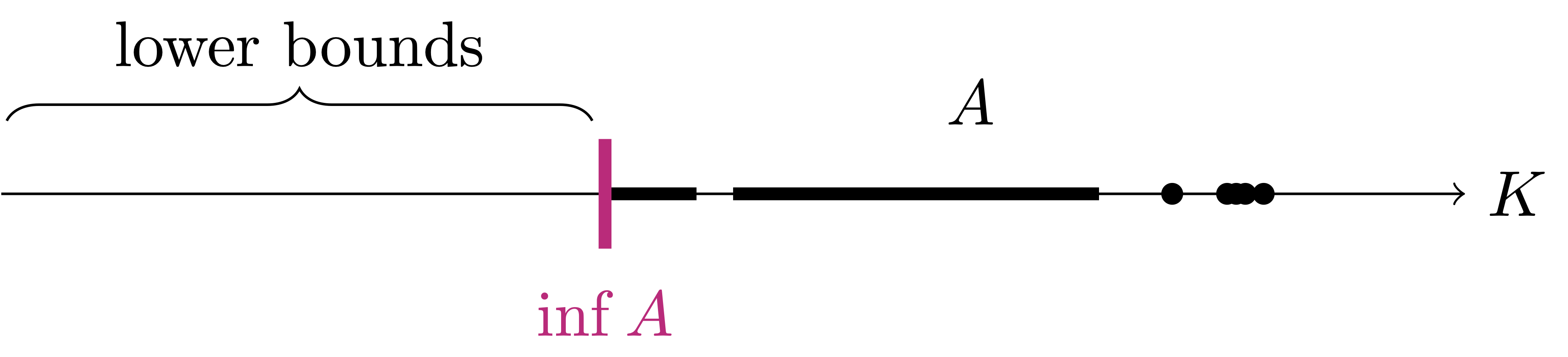
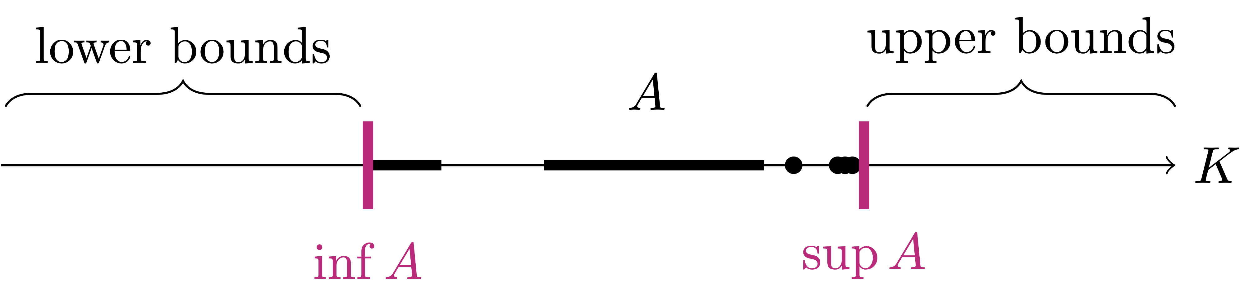
3.4.1 Upper bound, supremum, maximum
We start by defining the supremum. First we need the notion of upper bound of a set. In the following we assume that \((K,+,\cdot,\leq)\) is an ordered field.
Definition 26: Upper bound and bounded above
Let \(A \subseteq K\):
- We say that \(b \in K\) is an upper bound for \(A\) if \[ a \leq b \,, \quad \forall \, a \in A \,. \]
- We say that \(A\) is bounded above if there exists and upper bound \(b \in K\) for \(A\).
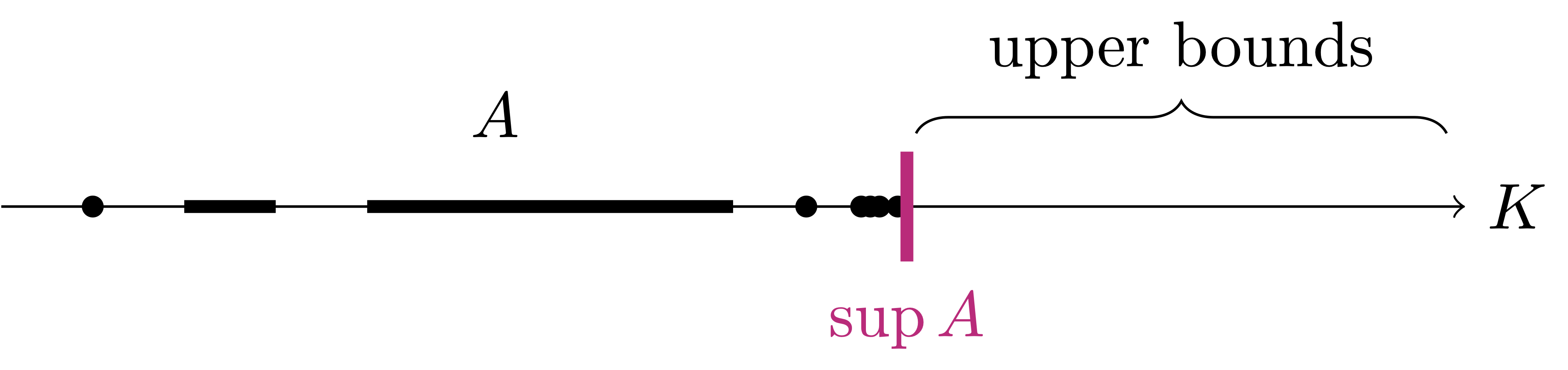
Definition 27: Supremum
- \(s\) is an upper bound for \(A\),
- \(s\) is the smallest upper bound of \(A\), that is, \[ \mbox{If } \, b \in K \, \mbox{ is upper bound for } \, A \, \mbox{ then } \, s \leq b \,. \]
If it exists, the supremum is denoted by \[ s := \sup \ A \,. \]
Remark 28
Proposition 29: Uniqueness of the supremum
Proof
- Since \(s_2 = \sup A\), in particular \(s_2\) is an upper bound for \(A\). Since \(s_1 = \sup A\) then \(s_1\) is the lowest upper bound. Thus we get \[ s_1 \leq s_2 \,. \]
- Exchanging the roles \(s_1\) and \(s_2\) in the above reasoning we also get \[ s_2 \leq s_1 \,. \]
This shows \(s_1 = s_2\).
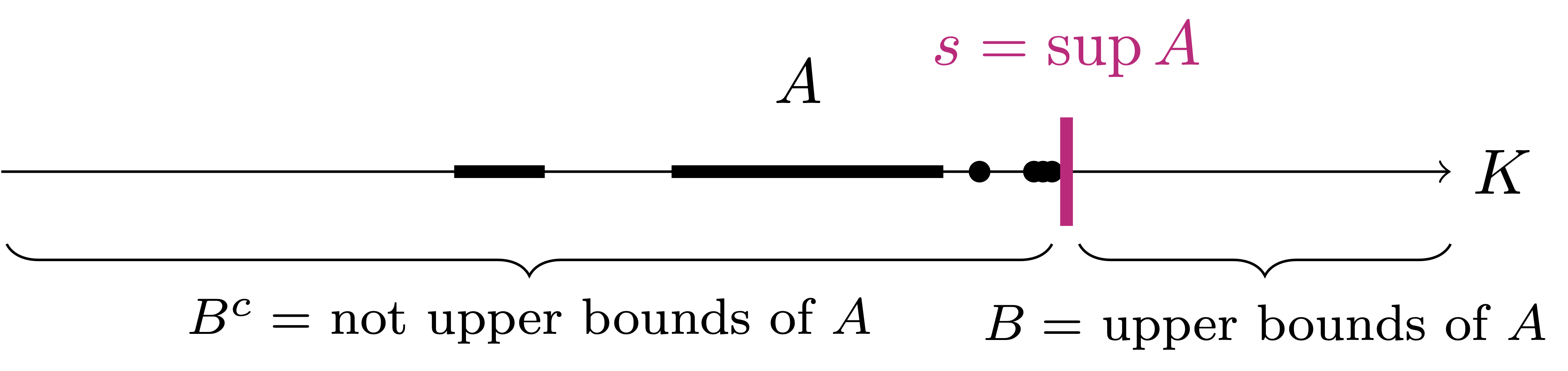
Warning
- A set can have infinite upper bounds,
- The supremum does not belong to the set.
For example \[ A = [0,1) \cap \mathbb{Q} \] has for upper bounds all the numbers \(b \in \mathbb{Q}\) with \(b>1\). Moreover one can show that \[ \sup A = 1\,, \] and so \[ \sup A \notin A \,. \]
Warning
Definition 30: Maximum
Proposition 31: Relationship between Max and Sup
Proof
- By definition we have \(M \in A\) and \[ a \leq M \,, \quad \forall \, a \in A \,. \] In particular the above tells us that \(M\) is an upper bound of \(A\).
- We claim that \(M\) is the least upper bound. Indeed, suppose \(b\) is an upper bound of \(A\), that is,
\[ a \leq b \,, \quad \forall \, a \in A \,. \] In particular, since \(M \in A\), by the above condition we have \[ M \leq b \,. \]
Therefore \(M\) is the least upper bound of \(A\), meaning that \(M = \sup A\).
Warning
3.4.2 Lower bound, infimum, minimum
We now introduce the definitions of lower bound, infimum, minimum. These are the counterpart of upper bound, supremum and maximum, respectively. In the following \((K,+,\cdot,\leq)\) is an ordered field.
Definition 32: Lower bound, bounded below, infimum, minimum
Let \(A \subseteq K\):
We say that \(l \in K\) is a lower bound for \(A\) if \[ l \leq a \,, \quad \forall \, a \in A \,. \]
We say that \(A\) is bounded below if there exists a lower bound \(l \in K\) for \(A\).
We say that \(i \in K\) is the greatest lower bound or infimum of \(A\) if:
- \(i\) is a lower bound for \(A\),
- \(i\) is the largest lower bound of \(A\), that is, \[ \mbox{If } \, l \in K \, \mbox{ is a lower bound for } \, A \, \mbox{ then } \, l \leq i \,. \] If it exists, the infimum is denoted by \[ i = \inf A \,. \]
We say that \(m \in K\) is the minimum of \(A\) if: \[ m \in A \,\, \mbox{ and } \,\, m \leq a \,, \, \forall a \in A \,. \] If it exists, we denote the minimum by \[ m = \min A \,. \]
Proposition 33
Let \(A \subseteq K\):
- If \(\inf A\) exists, then it is unique.
- If the minimum of \(A\) exists, then also the infimum exists, and \[ \inf A = \min A \,. \]
The proof is similar to the ones of Propositions 29 and 32, and is left to the reader as an exercise.
Warning
- A set has infinite lower bounds,
- The infimum does not belong to the set.
For example \[ A = (0,1) \cap \mathbb{Q} \] has for lower bounds all the numbers \(b \in \mathbb{Q}\) with \(b<1\). Moreover we will show that \[ \inf A = 0\,, \] and so \[ \inf A \notin A \,. \]
Warning
Warning
Proposition 34
The proof is trivial, and is left as an exercise. We now have a complete picture about supremum and infimum, see Figure 3.1.
We conclude with another simple, but useful proposition. The proof is again left to the reader.
Proposition 35: Relationship between sup and inf
Let \(A \subseteq K\). Define \[ - A := \{ - a \, \colon \,a \in A \} \,. \] They hold:
- If \(\sup A\) exists, then \(\inf A\) exists and \[ \inf(-A) = - \sup A \,. \]
- If \(\inf A\) exists, then \(\sup A\) exists and \[ \sup(-A) = - \inf A \,. \]
3.5 Completeness
In this section \((K,+,\cdot, \leq)\) denotes an ordered field.
Question 36
The answer to the above question is NO. Like we did with the Cut Property, the counterexample can be found in the set of rational numbers \(\mathbb{Q}\). A set bounded above for which the supremum does nor exist is, for example, \[ A = [0, \sqrt{2}) \cap \mathbb{Q}\,. \tag{3.15}\]
Theorem 37
There exists a set \(A \subseteq \mathbb{Q}\) such that
- \(A\) is non-empty,
- \(A\) is bounded above,
- \(\sup A\) does not exist in \(\mathbb{Q}\).
The proof uses similar ideas to those employed in demonstrating that \(\mathbb{Q}\) does not satisfy the Cut Property, see the proof of Theorem 22.
Proof
Step 1. \(A\) is bounded above.
Take \(b:=3\). Then \(b\) is an upper bound for \(A\). Indeed by definition \[
q^2 < 2 \,, \,\, q \geq 0 \,, \,\,\, \forall \, q \in A \,.
\] Therefore \[
q^2 < 2 < 9 \implies q^2 < 9 \implies q < 3 = b
\] for each \(q \in A\), showing that \(b=3\) is an upper bound for \(A\).
Step 2. The supremum of \(A\) does not exist in \(\mathbb{Q}\).
Assume by contradiction that there exists \[
s = \sup A \in \mathbb{Q}
\] By definition it holds \[
q \leq s \,, \quad \forall \, q \in A
\tag{3.16}\] \[
q \leq b \,, \, \forall \, q \in A \,\, \implies \,\,
s \leq b
\tag{3.17}\] There are two possibilities: \(s \in A\) or \(s \notin A\).
Case 1. If \(s \in A\), by definition of \(A\) we have \[ s \geq 0\,, \quad s^2 < 2 \,. \tag{3.18}\] Define \[ \widetilde{s} := s + \frac{1}{n} \] with \(n \in \mathbb{N}\), \(n \neq 0\) to be chosen later. Then \[\begin{align*} \widetilde{s}^2 & = \left( s + \frac1n \right)^2 \\ & = s^2 + \frac{1}{n^2} + 2 \frac{s}{n} \\ & < s^2 + \frac{1}{n} + 2 \frac{s}{n} \qquad \left(\mbox{using } \, \frac{1}{n}<\frac{1}{n^2} \right) \\ & = s^2 + \frac{2s + 1}{n} \,. \end{align*}\] If we now impose that \[ s^2 + \frac{2s + 1}{n} < 2 \,, \] we can rearrange the above and obtain \[ n(2 - s^2) > 2s + 1 \,. \] Now note that \(s^2 < 2\) by assumption (3.18). Thus we can divide by \((2 - s^2)\) and obtain \[ n >\frac{2s + 1}{2 - s^2} \,. \] To summarize, we have just shown that \[ n >\frac{2s + 1}{2 - s^2} \,\, \implies \,\, \widetilde{s}^2 < 2 \,. \] Moreover \(\widetilde{s} := (s + 1/n) \in \mathbb{Q}\) and \[ \tilde{s} > s \geq 0 \,, \] showing that \[ \widetilde{s} \in A \,. \] Since \(s = \sup A\), we then have \[ \widetilde{s} \leq s \,. \] However \[ \widetilde{s} := s + \frac{1}{n} > s \,, \] yielding a contradiction. Thus \(s \in A\) is not possible.
Case 2. Assume \(s \notin A\). Since \(s = \sup A\) and \(0 \in A\), we deduce that \[
s>0 \,.
\] In particular \(s \notin A\) implies that \[
s^2 > 2 \,.
\tag{3.19}\]
Define \[
\widetilde{s} := s - \frac{1}{n} \,.
\] We have \[\begin{align*}
\widetilde{s}^2 & = \left( s - \frac1n \right)^2 \\
& = s^2 + \frac{1}{n^2} - 2 \frac{s}{n} \\
& > s^2 - \frac{1}{n^2} - 2 \frac{s}{n} \qquad \left(\mbox{using } \, \frac{1}{n^2} > - \frac{1}{n^2} \right) \\
& > s^2 - \frac{1}{n} - 2 \frac{s}{n} \qquad \left(\mbox{using } \, -\frac{1}{n^2} > - \frac{1}{n} \right) \\
& = s^2 - \frac{1 + 2s}{n} \,.
\end{align*}\] Now we impose \[
s^2 - \frac{1 + 2s}{n} > 2
\] which is equivalent to \[
n(s^2 - 2) > 1 + 2s \,.
\] By (3.19) we have \(s^2 > 2\). Therefore we can divide by \((s^2 -2)\) and get \[
n > \frac{1+2s}{s^2 - 2} \,.
\] In summary, we have just shown that \[
n > \frac{1+2s}{s^2 - 2} \quad \implies \quad \widetilde{s}^2 > 2\,.
\] We also want to choose \(n\) in such a way that \[
\widetilde{s} > 0
\] This means \[
0 < \widetilde{s} = s - \frac1n \quad \iff \quad n > \frac{1}{s}
\] Therefore \[
n > \min \left\{ \frac{1+2s}{s^2 - 2}, \frac1s \right\} \quad \implies \quad \widetilde{s} > 0\,, \quad \widetilde{s}^2 > 2
\] In particular \(\widetilde{s} \notin A\), and by definition of \(A\) we have \[
\widetilde{s} \geq q \,, \quad \forall \, q \in A\,.
\]
Indeed, assume \(\widetilde{s} < q\) for some \(q \in A\). Since \(\widetilde{s}>0\), we can take the squares and deduce that \(\widetilde{s}^2<q^2<2\), which is a contradiction.
By definition we have \(\widetilde{s} = (s - 1/n) \in \mathbb{Q}\). Therefore \(\widetilde{s}\) is an upper bound for \(A\) in \(\mathbb{Q}\). Since \(s=\sup A\) is the smallest upper bound, see (3.17), it follows that \[ s \leq \widetilde{s} \,. \] However \[ \widetilde{s} := s - \frac{1}{n} < s \,, \] obtaining a contradiction. Then \(s \notin A\).
Conclusion. We have assumed by contradiction that \(s = \sup A\) exists in \(\mathbb{Q}\). In this case either \(s \in A\) or \(s \notin A\). In both instances we found a contradiction. Therefore \(\sup A\) does not exist in \(\mathbb{Q}\).
The above theorem shows that the supremum does not necessarily exist. What about the infimum?
Question 38
The answer to the above question is again NO. A set bounded below for which the infimum does nor exist is, for example, \[ A = (\sqrt{2}, 10] \cap \mathbb{Q}\,. \] The proof of this fact is, of course, very similar to the one of Theorem 48, and is therefore omitted.
In conclusion, infimum and supremum do not exist in general. The fields for which all bounded sets admit supremum or infimum are called complete.
Definition 39: Completeness
Let \((K,+,\cdot,\leq)\) be an ordered field. We say that \(K\) is complete if the following property holds:
- (AC) For every \(A \subseteq K\) non-empty and bounded above \[ \sup A \in K \,. \]
In particular, Theorem 48 can be re-stated as follows.
Theorem 40
- \(A\) is non-empty,
- \(A\) is bounded above,
- \(\sup A\) does not exist in \(\mathbb{Q}\).
One of such sets is, for example, \[ A = \{ q \in \mathbb{Q}\, \colon \,q \geq 0 \,, \,\, q^2 < 2 \} \,. \]
Notation 41
Property (AC) is called Axiom of Completeness
If \(K\) is an ordered field in which (AC) holds, then \(K\) is called a complete ordered field
Notice that if the Axiom of Completeness holds, then also the infimum exists. This is shown in the following proposition.
Proposition 42
Proof
Example 43
3.6 Equivalence of Completeness and Cut Property
We can show that Completeness is equivalent to the Cut Property.
Theorem 44: Equivalence of Cut Property and Completeness
Let \((K,+,\cdot, \leq)\) be an ordered field. They are equivalent:
- \(K\) has the Cut Property
- \(K\) is Complete
Remark 45: Ideas for proving Theorem 43
Step 1. Cut Property \(\implies\) Completeness.
Suppose \(K\) has the Cut Property. To prove that \(K\) is Complete, we need to:
Consider an arbitrary set \(A \subseteq K\) such that \(A \neq \emptyset\) and \(A\) is bounded above.
Show that \(A\) has a supremum.
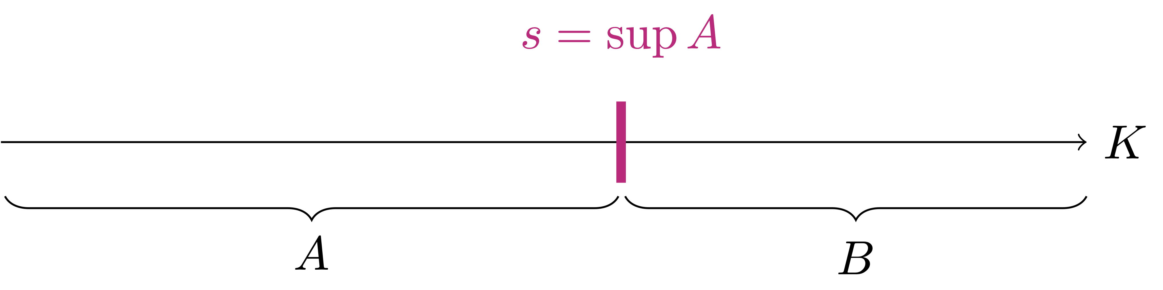
To achieve this, consider the set of upper bounds of \(A\) \[ B := \{ b \in K \, \colon \,b \geq a \,, \,\, \forall a \in A \} \,, \] We can show that the pair \[ (B^c,B) \] is a Cut of \(K\). As \(K\) has the Cut Property, then there exists \(s \in K\) separator of \((B^c,B)\). We will show that such separator \(s\) is the supremum of \(A\), i.e., \[ s = \sup A \,. \] This proves completeness of \(K\). See Figure 3.2 for a schematic picture of the above construction.
Step 2. Completeness \(\implies\) Cut Property.
Conversely, suppose that \(K\) is Complete. To prove that \(K\) has the Cut Property, we need to:
- Consider a cut \((A,B)\) of \(K\).
- Show that \((A,B)\) has a separator \(s \in K\).
This implication is easier. Indeed, since \(A\) is non-empty and bounded above (by the elements of \(B\)), by Completeness there exists \[ s:=\sup A \in K \,. \] We will show that \(s\) is a separator for the cut \((A,B)\), and therefore \(K\) has the Cut Property. See Figure 3.3 for a schematic picture of the above construction.
Keeping the above ideas in mind, let us proceed with the proof.
Proof: Proof of Theorem 43
We need to prove that \(K\) is complete. To this end, consider \(A \subseteq K\) non-empty and bounded above. Define the set of upper bounds of \(A\): \[ B := \{ b \in K \, \colon \,b \geq a \,, \,\, \forall a \in A \} \,. \]
Claim. The pair \((B^c,B)\) is a cut of \(K\).
Proof of Claim. We have to prove two points:
- \((B^c,B)\) forms a partition of \(K\).
Indeed, we have \(B \neq \emptyset\), since \(A\) is bounded above. Further, we have \(B^c \neq \emptyset\), since \(A\) is non-empty. Thus \[ K = B^c \cup B \,, \quad B^c \cap B = \emptyset \,. \] Then \((B^c,B)\) is a partition of \(K\).
- We have \[ x \leq y \,, \quad \forall \, x \in B^c\,, \,\forall \, y \in B \,. \tag{3.20}\]
To show the above, let \(x \in B^c\) and \(y \in B\). By definition of \(B\) we have that elements of \(B^c\) are not upper bounds of \(A\). Therefore \(x\) is not an upper bound. This means there exists \(\widetilde{a} \in A\) which is larger than \(x\), that is, \[ x \leq \widetilde{a} \,. \] Since \(y \in B\), then \(y\) is an upper bound for \(A\), so that \[ a \leq y \,, \,\, \forall a \in A\,. \] Therefore \[ x \leq \widetilde{a} \leq y \,, \] concluding (3.20).
Thus \((B^c,B)\) is a cut of \(K\) and the claim is proven.
Since \((B^c,B)\) is a cut of \(K\), by the Cut Property there exists a separator \(s \in K\) such that \[ x \leq s \leq y \,, \quad \forall \, x \in B^c\,, \,\forall \, y \in B \,. \tag{3.21}\]
Claim. \(s\) is an upper bound for \(A\).
Proof of Claim.
Suppose by contradiction that \(s\) is not an upper bound for \(A\). Therefore by definition of upper bound, there exists \(\widetilde{a} \in A\) such that \[
s < \widetilde{a} \,.
\] Consider the mid-point between \(s\) and \(\widetilde{a}\), that is, \[
m:=\frac{s + \widetilde{a}}{2} \in K \,.
\] Since \(m\) is the mid-point between \(s\) and \(\widetilde{a}\), and \(s < \widetilde{a}\), it holds \[
s < m < \widetilde{a} \,.
\]
Indeed, since \(s < \widetilde{a}\) then \[ s = \frac{2s}{2} < \frac{s + \widetilde{a}}{2} < \frac{2 \widetilde{a}}{2} = \widetilde{a} \,. \]
In particular the above tells us that \(m\) is not an upper bound for \(A\), given that \(\widetilde{a} \in A\) and \(m < \widetilde{a}\). Therefore \(m \in B^c\), by definition of \(B^c\). Therefore(3.21) implies \[ m \leq s \,, \] which contradicts \(s < m\). Hence \(s\) is an upper bound of \(A\), concluding the proof of Claim.
Conclusion. We have shown that \(s\) is an upper bound of \(A\). Condition
(3.21) tells us that \[
s \leq y \,, \,\, \forall y \in B \,.
\] Recalling that \(B\) is the set of upper bounds of \(A\), this means that \(s\) is the smallest upper bound of \(A\), that is, \[
s = \sup A \in K \,.
\]
Step 2. Completeness \(\implies\) Cut Property.
Suppose \(K\) is complete. We need to show that \(K\) has the Cut Property. Therefore assume \((A,B)\) is a cut of \(K\), that is, \[
A \neq \emptyset\,, \quad B \neq \emptyset \,,
\] \[
K = A \cup B\,, \quad A \cap B = \emptyset \,,
\] \[
a \leq b \,, \quad \forall a \in A \,, \,\, \forall \, b \in B \,.
\tag{3.22}\] Since \(B \neq \emptyset\), from (3.22) it follows that \(A\) is bounded above: indeed, every element of \(B\) is an upper bound for \(A\), thanks to (3.22). Since \(A \neq \emptyset\), by the Axiom of Completeness we have \[
s = \sup A \in K \,.
\] In particular, by definition of supremum, we have \[
a \leq s \,, \,\, \forall \, a \in A \,.
\] Let now \(b \in B\) be arbitrary. From (3.22) we have that \[
a \leq b \,, \,\, \forall \, a \in A \,.
\tag{3.23}\] Therefore \(b\) is an upper bound of \(A\). Since \(s = \sup A\), we have that \(s\) is the smallest upper bound, and so \[
s \leq b \,.
\] Given that \(b \in B\) was arbitrary, it actually holds \[
s \leq b \,, \,\, \forall \, b \in B \,.
\tag{3.24}\] From (3.23) and (3.24) we therefore have \[
a \leq s \leq b \,, \,\, \forall a \in A \,, \, \forall \, b \in B \,,
\] showing that \(s\) is a separator of \((A,B)\). Thus \(K\) has the Cut Property.
3.7 Axioms of Real Numbers
We now have all the key elements to introduce the Real Numbers \(\mathbb{R}\). These ingredients are:
- Definition of ordered field,
- The Cut Property or Axiom of Completeness.
The definition of \(\mathbb{R}\) is given in an axiomatic way.
Definition 46: System of Real Numbers \(\mathbb{R}\)
A system of Real Numbers is a set \(\mathbb{R}\) with two operations \(+\) and \(\cdot\), and a total order relation \(\leq\), such that
\((\mathbb{R},+,\cdot, \leq)\) is an ordered field
\(\mathbb{R}\) sastisfies the Axiom of Completeness
For reader’s convenience we explicitly state the above mentioned properties.
- There is an operation \(+\) of addition on \(\mathbb{R}\) \[
+\ \colon \mathbb{R}\times \mathbb{R}\to \mathbb{R}\,, \quad (x,y) \mapsto x + y
\] The addition satisifes: \(\,\forall \, x,y,z \in \mathbb{R}\)
- (A1) Commutativity and Associativity: \[ x+y = y+x \] \[ (x+y)+z = x+(y+z) \]
- (A2) Additive Identity: \(\,\exists \, 0 \in \mathbb{R}\, \text{ s.t. } \, \) \[ x + 0 = 0 + x = x \]
- (A3) Additive Inverse: \(\, \exists \, (-x) \in \mathbb{R}\, \text{ s.t. } \, \) \[ x + (-x) = (-x) + x = 0 \]
- There is an operation \(\cdot\) of multiplication on \(\mathbb{R}\) \[
\cdot\ \colon \mathbb{R}\times \mathbb{R}\to \mathbb{R}\,, \quad (x,y) \mapsto x \cdot y = xy
\] The multiplication satisifes: \(\, \forall \, x,y,z \in \mathbb{R}\)
- (M1) Commutativity and Associativity: \[ x \cdot y = y \cdot x \] \[ (x \cdot y) \cdot z = x \cdot (y \cdot z) \]
- (M2) Multiplicative Identity: \(\, \exists \, 1 \in \mathbb{R}\, \text{ s.t. } \, \) \[ x \cdot 1 = 1 \cdot x = x \]
- (M3) Multiplicative Inverse: If \(x \neq 0 \,, \,\, \exists \, x^{-1} \in \mathbb{R}\, \text{ s.t. } \, \) \[ x \cdot x^{-1} = x^{-1} \cdot x = 1 \]
- There is a relation \(\leq\) of total order on \(\mathbb{R}\). The order satisfies: \(\, \forall \, x, y, z \in \mathbb{R}\)
- (O1) Reflexivity: \[ x \leq x \]
- (O2) Antisymmetry: \[ x \leq y \, \mbox{ and } \, y \leq x \,\, \implies \,\, x = y \]
- (O3) Transitivity: \[ x \leq y \,\, \mbox{ and } \,\, y \leq z \,\, \implies \,\, x = z \]
- (O4) Total order:
\[ x \leq y \,\, \mbox{ or } \,\, y \leq x \]
- The operations \(+\) and \(\cdot\), and the total order \(\leq\), are related by the following properties: \(\, \forall x, y, z \in \mathbb{R}\)
- (AM) Distributive: Relates addition and multiplication via \[ x \cdot (y + z) = x \cdot y + x \cdot z \]
- (AO) Relates addition and order with the requirement: \[ x \leq y \,\, \implies \,\, x + z \leq y + z \]
- (MO) Relates multiplication and order with the requirement: \[ x \geq 0, \, y \geq 0 \,\, \implies \,\, x \cdot y \geq 0 \]
- Axiom of Completeness:
- (AC) For every \(A \subseteq \mathbb{R}\) non-empty and bounded above, there exists \[ \sup A \in \mathbb{R} \]
Remark 47
Since Axiom of Completeness and Cut Property are equivalent by Theorem 43, one can replace the Axiom of Completeness in Definition 45 Point 5 with:
- Cut Property holds:
- (CP) Every cut \((A,B)\) of \(\mathbb{R}\) admits a separator \(s \in \mathbb{R}\, \, \text{ s.t. } \, \) \[ a \leq s \leq b \,, \quad \forall \, a \in A \,, \,\forall \, b \in B \]
Notation 48
Remark 49
\((K,+,\cdot)\) is a field if they hold: \[ \mbox{(A1)-(A3), (M1)-(M3), (AM)} \]
\((K,+,\cdot, \leq)\) is an ordered field if they hold \[ \mbox{(A1)-(A3), (M1)-(M3), (O1)-(O4) ,(AM), (AO), (MO)} \]
In particular we have that \[ (\mathbb{R},+, \cdot,\leq) \] is a complete ordered field: that is, an ordered field in which the Cut Property (CP) or Axiom of Completeness (AC) hold.
Question 50
There are two main questions here:
We have only postulated the existence of \(\mathbb{R}\). Does such complete ordered field actually exist?
Is \(\mathbb{R}\) the only complete ordered field?
The answer to both questions is YES:
There are several equivalent methods for explicitly constructing the system \(\mathbb{R}\). One such method uses Dedekind cuts. The interested reader can refer to the Appendix in Chapter 1 of (Rudin 1976), or Chapter 8.6 in (Abbott 2015).
It can be shown that \((\mathbb{R},+, \cdot,\leq)\) is the only complete ordered field. Uniqueness is intended in the following sense: if \((K,+, \cdot,\leq)\) is another complete ordered field, then \(K\) looks like \(\mathbb{R}\). Mathematically this means that there exists an invertible map \(\Psi \ \colon \mathbb{R}\to K\), called isomorphism of fields, which preserves the operations \(+\), \(\cdot\) and the order \(\leq\).
In particular the following Theorem can be proven.
Theorem 51: Existence of the Real Numbers
3.8 Special subsets of \(\mathbb{R}\)
In Definition 45, we introduced \(\mathbb{R}\) as a complete ordered field, doing so axiomatically and in a non-constructive manner. But what about the sets \(\mathbb{N}\), \(\mathbb{Z}\), \(\mathbb{Q}\) now? Are they still well-defined? Specifically, can we say that \[ \mathbb{N}\,, \mathbb{Z}\,, \mathbb{Q}\, \subseteq \mathbb{R}\,? \] The definitions we provided in Chapter 1 for \(\mathbb{N}\), \(\mathbb{Z}\), and \(\mathbb{Q}\) are not directly linked to the real number system \(\mathbb{R}\) we just introduced. To address this issue, we will need to define new sets \[ \mathbb{N}_{\mathbb{R}}, \,\, \mathbb{Z}_{\mathbb{R}}\,, \,\, \mathbb{Q}_{\mathbb{R}} \] from scratch, relying solely on the axioms of \(\mathbb{R}\). The subscript \(\mathbb{R}\) is used here to clearly distinguish these new sets from the original ones.
3.8.1 Natural numbers
Let us start with the definition of \({\mathbb{N}}_{\mathbb{R}}\). We would like \({\mathbb{N}}_{\mathbb{R}}\) to be \[ {\mathbb{N}}_{\mathbb{R}} = \{ \mathbf{1}, \mathbf{2} , \mathbf{3} , \ldots \} \,. \] We are denoting the above numbers with bold symbols in order to distinguish them from the elements of \(\mathbb{R}\). The key property that we would like \({\mathbb{N}}_{\mathbb{R}}\) to have is the following: \[ \mbox{Every } \mathbf{n} \in {\mathbb{N}}_{\mathbb{R}} \, \mbox{ has a successor } \, (\mathbf{n+1}) \in {\mathbb{N}}_{\mathbb{R}} \,. \] How do we ensure this property? We could start by defining \[ \mathbf{1}:=1\,, \] with \(1\) the neutral element of the multiplication in \(\mathbb{R}\), which exists by the field axiom (M2) in Defintion 45. We could then define \(\mathbf{2}\) by setting \[ \mathbf{2} := 1 + 1 \,. \] We need a formal definition to capture this idea.
Definition 52: Inductive set
Let \(S \subseteq \mathbb{R}\). We say that \(S\) is an inductive set if they are satisfied:
- \(1 \in S\),
- If \(x \in S\), then \((x + 1) \in S\).
Note that in the above definition we just used:
- The existence of the neutral element \(1\), given by axiom (M2).
- The operation of sum in \(\mathbb{R}\), which is again given as an axiom.
Example 53
Question. Prove the following:
\(\mathbb{R}\) is an inductive set.
The set \(A=\{0,1\}\) is not an inductive set.
Solution.
We have that \(1 \in \mathbb{R}\) by axiom (M2). Moreover \((x + 1) \in \mathbb{R}\) for every \(x \in \mathbb{R}\), by definition of sum \(+\).
We have \(1 \in A\), but \((1 + 1) \notin A\), since \(1 + 1 \neq 0\).
Since \(\mathbb{R}\) is itself an inductive set, it is clear that the definition of inductive set is not sufficient to fully describe our intuitive idea of \({\mathbb{N}}_{\mathbb{R}}\). The right way to define \({\mathbb{N}}_{\mathbb{R}}\) is as follows: \[ {\mathbb{N}}_{\mathbb{R}} \mbox{ is the smallest inductive subset of } \mathbb{R}\,. \] To make the above definition precise, we first need a Proposition.
Proposition 54
Proof
We have \(1 \in M\) for every \(M \in \mathcal{M}\), since these are inductive sets. Thus \[ 1 \in \bigcap_{M \in \mathcal{M}} \, M = S \,. \]
Suppose that \(x \in S\). By definition of \(S\) this implies that \(x \in M\) for all \(M \in \mathcal{M}\). Since \(M\) is an inductive set, then \((x + 1) \in M\). Therefore \((x+1) \in M\) for all \(M \in \mathcal{M}\), showing that \((x+1) \in S\).
Therefore \(S\) is an inductive set.
We are now ready to define the natural numbers \({\mathbb{N}}_{\mathbb{R}}\).
Definition 55: Set of Natural Numbers
Therefore \({\mathbb{N}}_{\mathbb{R}}\) is the intersection of all the inductive subsets of \(\mathbb{R}\). From this definition it follows that \({\mathbb{N}}_{\mathbb{R}}\) is the smallest inductive subset of \(\mathbb{R}\), as shown in the following Proposition.
Proposition 56: \({\mathbb{N}}_{\mathbb{R}}\) is the smallest inductive subset of \(\mathbb{R}\)
Proof
The definition of \({\mathbb{N}}_{\mathbb{R}}\) guarantees that all numbers in \({\mathbb{N}}_{\mathbb{R}}\) are larger than \(1\).
Theorem 57
Proof
By definition \(1 \in C\). Suppose now that \(x \in C\), so that \(x \geq 1\). Since \(1 \geq 0\) as a consequence of the field axioms, we deduce that \[ x + 1 \geq x + 0 = x \geq 1 \,, \] showing that \(x + 1 \geq 1\). Thus \((x + 1) \in C\).
By Proposition 56 we conclude that \[ {\mathbb{N}}_{\mathbb{R}} \subseteq C \,, \] showing that \(x \geq 1\) for all \(x \in {\mathbb{N}}_{\mathbb{R}}\).
Notation 58
3.8.2 Principle of induction
The Principle of Induction is a consequence of the definition of \({\mathbb{N}}_{\mathbb{R}}\), see Definition 54, and of the field axioms of \(\mathbb{R}\) in Definition 45.
Theorem 59: Principle of Induction
- \(\alpha(1)\) is true.
- If \(\alpha(n)\) is true then also \(\alpha(n+1)\) is true.
Then \(\alpha(n)\) is true for all \(n \in {\mathbb{N}}_{\mathbb{R}}\).
Proof
Indeed:
- \(1 \in C\) since \(\alpha(1)\) is true by assumption.
- If \(n \in C\) then \(\alpha(n)\) is true. By assumption \(\alpha(n+1)\) is true. Therefore \((n+1) \in C\).
By Proposition 56 we conclude that \[ {\mathbb{N}}_{\mathbb{R}} \subseteq C\,. \] As by definition \(C \subseteq {\mathbb{N}}_{\mathbb{R}}\), we have proven that \[ {\mathbb{N}}_{\mathbb{R}} = C \,, \] showing that \(\alpha(n)\) is true for all \(n \in {\mathbb{N}}_{\mathbb{R}}\).
As a consequence of the principle of induction, we can prove that \({\mathbb{N}}_{\mathbb{R}}\) is closed under the field operations of sum and multiplication.
Theorem 60
For all \(n,m \in {\mathbb{N}}_{\mathbb{R}}\) we have:
\({\mathbb{N}}_{\mathbb{R}}\) is closed under addition, that is, \[ m + n \in {\mathbb{N}}_{\mathbb{R}} \,. \]
\({\mathbb{N}}_{\mathbb{R}}\) is closed under multiplication, that is, \[ m \cdot n \in {\mathbb{N}}_{\mathbb{R}} \,, \]
If \(m > n\) there exists \(k \in {\mathbb{N}}_{\mathbb{R}}\) such that \[ m = n + k \,. \]
Proof
- Induction base: We have \(m+1 \in {\mathbb{N}}_{\mathbb{R}}\), since \(m \in {\mathbb{N}}_{\mathbb{R}}\) and \({\mathbb{N}}_{\mathbb{R}}\) is an inductive set.
- Inductive hypothesis: Suppose \(m+n \in {\mathbb{N}}_{\mathbb{R}}\). Since \({\mathbb{N}}_{\mathbb{R}}\) is an inductive set, we have \((m+n)+ 1 \in {\mathbb{N}}_{\mathbb{R}}\). By associativity of the sum, see axiom (A1), we get \[ m + (n + 1) = ( m + n ) + 1 \in {\mathbb{N}}_{\mathbb{R}} \,, \] which is the desired theis.
By the Induction Principle of Theorem 58 we conclude (3.25).
As a consequence of the above theorem, we see that the restriction of the operations of sum and multiplication to \({\mathbb{N}}_{\mathbb{R}}\) are still binary operations: \[ + \, \colon {\mathbb{N}}_{\mathbb{R}} \times {\mathbb{N}}_{\mathbb{R}} \to {\mathbb{N}}_{\mathbb{R}} \,, \quad \cdot \, \colon {\mathbb{N}}_{\mathbb{R}} \times {\mathbb{N}}_{\mathbb{R}} \to {\mathbb{N}}_{\mathbb{R}} \,. \]
Equipped with the above operations, \({\mathbb{N}}_{\mathbb{R}}\) satisfies the following properties.
Theorem 61
\(({\mathbb{N}}_{\mathbb{R}}, + , \cdot, \leq )\) satisfies the following axioms from Definition 45:
- (A1).
- (M1), (M2).
- (O1)-(O4).
- (AM), (AO), (MO).
The proof is trivial, as it follows immediately from the inclusion of \({\mathbb{N}}_{\mathbb{R}}\) in \(\mathbb{R}\).
3.8.3 Integers
We have seen in Theorem 60 that \({\mathbb{N}}_{\mathbb{R}}\) is closed under addition. However \({\mathbb{N}}_{\mathbb{R}}\) is not closed under subtraction. We therefore define the set of integers \({\mathbb{Z}}_{\mathbb{R}}\) in a way that we can perform subtraction of any two natural numbers.
Definition 62: Set of Integers
In the definition of \({\mathbb{Z}}_{\mathbb{R}}\) we denote by \(-n\) the inverse of \(n\) in \(\mathbb{R}\), which exists by the field axiom (A3) in Definition 45. The following characterization explains the relationship between \({\mathbb{Z}}_{\mathbb{R}}\) and \({\mathbb{N}}_{\mathbb{R}}\).
Theorem 63
Proof
\(M \subseteq {\mathbb{Z}}_{\mathbb{R}}\): Suppose \(m \in M\). We have 3 cases:
- If \(m \in \{ -n \, \colon \,n \in {\mathbb{N}}_{\mathbb{R}}\}\) then there exists \(n \in {\mathbb{N}}_{\mathbb{R}}\) such that \(m=-n\). Thus \[ m = -n = 1 - (n+1) \in {\mathbb{Z}}_{\mathbb{R}} \,, \] since \(1 \in {\mathbb{N}}_{\mathbb{R}}\) and \(n+1 \in {\mathbb{N}}_{\mathbb{R}}\) because \(n \in {\mathbb{N}}_{\mathbb{R}}\).
- If \(m=0\) then \[ m = 0 = 1 - 1 \in {\mathbb{Z}}_{\mathbb{R}}\,, \] as \(1 \in {\mathbb{N}}_{\mathbb{R}}\).
- If \(m \in {\mathbb{N}}_{\mathbb{R}}\) then \[ m = (m + 1) - 1 \in {\mathbb{Z}}_{\mathbb{R}} \,, \] since \(1 \in {\mathbb{N}}_{\mathbb{R}}\) and \(m+1 \in {\mathbb{N}}_{\mathbb{R}}\), given that \(m \in {\mathbb{N}}_{\mathbb{R}}\).
In all 3 cases we have shown that \(m \in {\mathbb{Z}}_{\mathbb{R}}\), proving that \(M \subseteq {\mathbb{Z}}_{\mathbb{R}}\).
\({\mathbb{Z}}_{\mathbb{R}} \subseteq M\): Let \(z \in {\mathbb{Z}}_{\mathbb{R}}\). Then \(z = m - n\) for some \(n,m \in {\mathbb{N}}_{\mathbb{R}}\). We have 3 cases:
- If \(m=n\) then \[ z = m - n = m - m \stackrel{(A3)}{=} 0 \in M \,. \]
- If \(m>n\), by Theorem 60 there exists \(k \in {\mathbb{N}}_{\mathbb{R}}\) such that \(m = k + n\). Therefore \[\begin{align*} z & = m - n = (k + n) - n \\ & \stackrel{(A1)}{=} k + (n-n) \stackrel{(A3)}{=} k + 0 \\ & \stackrel{(A2)}{=} k \in M \,, \end{align*}\] since \(k \in {\mathbb{N}}_{\mathbb{R}}\).
- If \(m<n\), by Theorem 60 there exists \(k \in {\mathbb{N}}_{\mathbb{R}}\) such that \(n = k + m\). Therefore \[ z = m - n = - k \in M \,, \] since \(k \in {\mathbb{N}}_{\mathbb{R}}\), where again we have used (implicitly) the field axioms (A1), (A2) and (A3).
Therefore \({\mathbb{Z}}_{\mathbb{R}} = M\).
Like we did with \({\mathbb{N}}_{\mathbb{R}}\), we can also show that \({\mathbb{Z}}_{\mathbb{R}}\) is closed under the operations of sum and multiplication.
Theorem 64
For all \(n,m \in {\mathbb{Z}}_{\mathbb{R}}\) we have:
\({\mathbb{Z}}_{\mathbb{R}}\) is closed under addition, that is, \[ m + n \in {\mathbb{Z}}_{\mathbb{R}} \,. \]
\({\mathbb{Z}}_{\mathbb{R}}\) is closed under multiplication, that is, \[ m \cdot n \in {\mathbb{Z}}_{\mathbb{R}} \,, \]
The proof is left as an exercise. As a consequence of Theorem 64 we have that the restriction of the operations of sum and multiplication to \({\mathbb{Z}}_{\mathbb{R}}\) are still binary operations: \[ + \, \colon {\mathbb{Z}}_{\mathbb{R}} \times {\mathbb{Z}}_{\mathbb{R}} \to {\mathbb{Z}}_{\mathbb{R}} \,, \quad \cdot \, \colon {\mathbb{Z}}_{\mathbb{R}} \times {\mathbb{Z}}_{\mathbb{R}} \to {\mathbb{Z}}_{\mathbb{R}} \,. \]
Equipped with the above operations, \({\mathbb{Z}}_{\mathbb{R}}\) satisfies the following properties.
Theorem 65
\(({\mathbb{Z}}_{\mathbb{R}}, + , \cdot, \leq )\) satisfies the following axioms from Definition 45:
- (A1), (A2), (A3).
- (M1), (M2).
- (O1)-(O4).
- (AM), (AO), (MO).
Proof
Remark 66
\({\mathbb{Z}}_{\mathbb{R}}\) does not satisfy (M3).
For example, let us show that \(2 \in {\mathbb{Z}}_{\mathbb{R}}\) has no inverse in \({\mathbb{Z}}_{\mathbb{R}}\). Indeed, let \(m \in {\mathbb{Z}}_{\mathbb{R}}\). By Theorem 63 we have 3 cases:
\(m \in {\mathbb{N}}_{\mathbb{R}}\): Since \(2 > 1\) we have \[ 2 \cdot m > 1 \cdot m \geq 1 \] where in the last inequality we used that \(m \geq 1\) for all \(m \in {\mathbb{N}}_{\mathbb{R}}\), as shown in Theorem 56. The above shows that \[ 2 \cdot m > 1\,, \] and therefore \(m\) cannot be the inverse of \(2\).
\(m=0\): Then \(2 \cdot m = 0\), so that \(m\) cannot be the inverse of \(2\).
\(m = -n\) with \(n \in {\mathbb{N}}_{\mathbb{R}}\). Then \[ 2 \cdot m = 2 \cdot (-n) < 0 \,, \] so that \(m\) cannot be the inverse of \(2\).
As we have exhausted all the possibilities, we conclude that \(2\) does not have a multiplicative inverse in \({\mathbb{N}}_{\mathbb{R}}\).
3.8.4 Rational numbers
In Theorem 65 and 66 we have seen that \({\mathbb{Z}}_{\mathbb{R}}\) satisfy all the field axiom, except for (M3). We therefore extend \({\mathbb{Z}}_{\mathbb{R}}\) in a way that the extension contains multiplicative inverses. The extension is the set of rational numbers \({\mathbb{Q}}_{\mathbb{R}}\).
Definition 67: Set of Rational Numbers
Notice that in the above definition we are just using the field axiom (M3), with \[ \frac{m}{n} := m \cdot n^{-1} \,. \] The inverse of \(n\) exists because we are assuming \(n \in {\mathbb{N}}_{\mathbb{R}}\), and therefore \(n\) cannot be \(0\), as a consequence of Theorem 56.
The set \({\mathbb{Q}}_{\mathbb{R}}\) is closed under addition and multiplication (exercise). Therefore they are well defined the operations: \[ + \, \colon {\mathbb{Q}}_{\mathbb{R}} \times {\mathbb{Q}}_{\mathbb{R}} \to {\mathbb{Q}}_{\mathbb{R}} \,, \quad \cdot \, \colon {\mathbb{Q}}_{\mathbb{R}} \times {\mathbb{Q}}_{\mathbb{R}} \to {\mathbb{Q}}_{\mathbb{R}} \,. \]
Theorem 68
Proof
- \(m>0\): In this case \(m \in {\mathbb{N}}_{\mathbb{R}}\) by Theorem 63. Therefore \[ p = \frac{n}{m} \in {\mathbb{Q}}_{\mathbb{R}} \] by definition, since \(n,m \in {\mathbb{N}}_{\mathbb{R}}\). By commutativity we have \[ q \cdot p = \frac{m}{n} \cdot \frac{n}{m} = 1 \,. \]
- \(m<0\): Then \(m=-x\) with \(x \in {\mathbb{N}}_{\mathbb{R}}\) by Theorem 63. Therefore \[ p = \frac{-n}{x} \in {\mathbb{Q}}_{\mathbb{R}} \] by definition, since \(-n \in {\mathbb{Z}}_{\mathbb{R}}\) and \(x \in {\mathbb{N}}_{\mathbb{R}}\). By commutativity we have \[ q \cdot p = \frac{m}{n} \cdot \frac{-n}{x} = \frac{m}{n} \cdot \frac{-n}{-m} = 1 \,. \]
Therefore \(q\) always admits a multiplicative inverse \(q^{-1}\) belonging to \({\mathbb{Q}}_{\mathbb{R}}\), proving (M3).
The set \({\mathbb{Q}}_{\mathbb{R}}\) does not have the Cut Property or the Axiom of Completeness.
Theorem 69
The proof of the above Theorem replicates exactly the proof of Theorem 48: This is because the proof of Theorem 48 only makes use of field axioms, and thus it applies to \({\mathbb{Q}}_{\mathbb{R}}\).