5  Complex Numbers

In Section 4.4, we have proven the existence of $\sqrt{x}$ for all for $x\ge 0$. The number $\sqrt{x}$ was defined as $$\sqrt{x}:=\alpha ,\alpha :=sup\{t\in \mathbb{R}:t^2<x\}.$$ We then proved that $${\alpha }^2=x.$$ This procedure is possible for any $x\ge 0$.

Question 1

Is there a number $\alpha \in \mathbb{R}$ such that $$\begin{array}{}\text{(5.1)}& {\alpha }^2=-1?\end{array}$$

The answer to the above question is no. This is because $\mathbb{R}$ is an ordered field, and from axiom (MO) it follows that: $$x^2\ge 0,\mathrm{\forall }x\in \mathbb{R}.$$ However we would still like to solve equation (5.1) somehow. To do this, we introduce the imaginary numbers or complex numbers. We define $i$ to be that number such that $$i^2=-1.$$ Formally, we can also think of $i$ as $$i=\sqrt{-1}.$$ We can use this speacial number to define the square root of a negative real number $x<0$: $$\sqrt{x}:=i\sqrt{-x}.$$ Note that $\sqrt{-x}$ is properly defined in $\mathbb{R}$, because $-x$ is positive when $x$ is negative.

5.1 The field $\mathbb{C}$

We would like to be able to do calculations with the newly introduced complex numbers, and investigate their properties. We can introduce them rigorously as a field, as we did for $\mathbb{R}$.

Definition 2: Complex Numbers

The set of complex numbers $\mathbb{C}$ is defined as

$$\mathbb{C}:=\mathbb{R}\oplus i\mathbb{R}:=\{x\oplus iy:x,y\in \mathbb{R}\}.$$

In the above the symbol $\oplus$ is used to denote the pair $$x\oplus iy=(x,y)$$ with $x,y\in \mathbb{R}$. This means that $x$ and $y$ play different roles.

Definition 3

For a complex number $$z=x\oplus iy\in \mathbb{C}$$ we say that

• $x$ is the real part of $z$, and denote it by $$x=\mathrm{Re}(z)$$
• $y$ is the imaginary part of $z$, and denote it by $$y=\mathrm{Im}(z)$$

We say that

• If $\mathrm{Re}z=0$ then $z$ is a purely imaginary number.
• If $\mathrm{Im}z=0$ then $z$ is a real number.

In order to make the set $\mathbb{C}$ into a field, we first have to define the two binary operations of addition $+$ and multiplication $\cdot$, $$+,\cdot :\mathbb{C}\times \mathbb{C}\to \mathbb{C}.$$ Then we need to prove that these operations satisfy all the field axioms.

Definition 4: Addition in $\mathbb{C}$

Let $z_1,z_2\in \mathbb{C}$, so that $$z_1=x_1\oplus i{y}_1,z_2=x_2\oplus i{y}_2,$$ for some $x_1,x_2,y_1,y_2\in \mathbb{R}$. We define the sum of $z_1$ and $z_2$ as $$z_1+z_2=(x_1\oplus i{y}_1)+(x_2\oplus i{y}_2):=(x_1+x_2)\oplus i(y_1+y_2)$$ where the $+$ symbol on the right hand side is the addition operator in $\mathbb{R}$.

Clearly, $z_1+z_2$ as defined above is an element of $\mathbb{C}$. Therefore $+$ defines a binary operation over $\mathbb{C}$.

Notation 5

From the above definition, we have that, for all $x,y\in \mathbb{R}$,

$$(x\oplus i0)+(0\oplus iy)=x\oplus iy.$$ To simplify notation, we will write $$x\oplus i0=x,0\oplus iy=iy$$ and $$x\oplus iy=x+iy.$$ We will also often swap $i$ and $y$, writing equivalently $$x+iy=x+yi.$$

We now want to define multiplication between complex numbers.

Remark 6: Formal calculation for multiplication in $\mathbb{C}$

How to define multiplication in $\mathbb{C}$? Whatever the definition may be, at least it has to give that that $$i^2=i\cdot i=-1.$$ Keeping the above in mind, let us do some formal calculations: For $z_1=x_1+i{y}_1,z_2=x_2+i{y}_2$ we have

$$\begin{array}{rl}{z}_1\cdot z_2& =(x_1+i{y}_1)\cdot (x_2+i{y}_2)\\ & =x_1\cdot x_2+x_1\cdot i{y}_2+x_2\cdot i{y}_1+y_1\cdot i^2{y}_2\\ & =(x_1\cdot x_2-y_1\cdot y_2)+i(x_1\cdot y_2+x_2\cdot y_1)\end{array}$$

Remark 6 motivates the following definition of multiplication.

Definition 7: Multiplication in $\mathbb{C}$

Let $z_1,z_2\in \mathbb{C}$, so that $$z_1=x_1\oplus i{y}_1,z_2=x_2\oplus i{y}_2,$$ for some $x_1,x_2,y_1,y_2\in \mathbb{R}$. Define the multiplication of $z_1$ and $z_2$ as $$\begin{array}{rl}{z}_1\cdot z_2& =(x_1+i{y}_1)\cdot (x_2+i{y}_2)\\ & :=(x_1\cdot x_2-y_1\cdot y_2)+i(x_1\cdot y_2+x_2\cdot y_1),\end{array}$$ where the operations $+$ and $\cdot$ on the right hand side are the operations in $\mathbb{R}$.

Clearly, $z_1\cdot z_2$ as defined above is an element of $\mathbb{C}$. Therefore $\cdot$ defines a binary operation over $\mathbb{C}$.

Remark 8

To check that we have given a good definition of product, we should have that $$i^2=-1,$$ as expected. Indeed:

$$\begin{array}{rl}{i}^2& =(0+1i)\cdot (0+1i)\\ & =(0\cdot 0-1\cdot 1)+(0\cdot 1+0\cdot 1)i=-1.\end{array}$$

Important

In view of Remark 8, we see that he formal calculations in Remark 6 are compatible with the definition of multiplication of complex numbers. Therefore, it is not necessary to memorize the multiplication formula, but it suffices to carry out calculations as usual, and replace $i^2$ by $-1$.

Example 9

Question. Compute $zw$, where $$z=-2+3i,w=1-i.$$

Solution. Using the definition we compute $$\begin{array}{rl}z\cdot w& =(-2+3i)\cdot (1-i)\\ & =(-2-(-3))+(2+3)i\\ & =1+5i.\end{array}$$ Alternatively, we can proceed formally as in Remark 6. We just need to recall that $i^2$ has to be replaced with $-1$: $$\begin{array}{rl}z\cdot w& =(-2+3i)\cdot (1-i)\\ & =-2+2i+3i-3i^2\\ & =(-2+3)+(2+3)i\\ & =1+5i.\end{array}$$

We now want to check that $$(\mathbb{C},+,\cdot )$$ is a field. All the field axioms are trivial to check, except for the existence of additive and multiplicative inverses.

Proposition 10: Additive inverse in $\mathbb{C}$

The neutral element of addition in $\mathbb{C}$ is the number $$0:=0+0i.$$ For any $z=x+iy\in \mathbb{C}$, the unique additive inverse is given by $$-z:=-x-iy.$$

The proof is immediate and is left as an exercise. The multiplication requires more care.

Remark 11: Formal calculation for multiplicative inverse

Let us first carry our some formal calculations. Let $$z=x+iy\in \mathbb{C},z\ne 0.$$ First, note that $$z\cdot 1=(x+iy)\cdot (1+0i)=x+iy=z,$$ and therefore $1$ is the neutral element of multiplication. Thus, the inverse of $z$ should be a complex number $z^{-1}\in \mathbb{C}$ such that $$z\cdot z^{-1}=1.$$ We would like to define $$z^{-1}=\frac{1}{x+iy}.$$ Such number does not belong to $\mathbb{C}$, as it is not of the form $a+ib$ for some $a,b\in \mathbb{R}$. However it is what the inverse should look like. Proceeding formally: $$\begin{array}{rl}\frac{1}{x+iy}& =\frac{1}{x+iy}\cdot 1\\ & =\frac{1}{x+iy}\cdot \frac{x-iy}{x-iy}\\ & =\frac{x-iy}{x^2-(iy{)}^2}\\ & =\frac{x-iy}{x^2+y^2}\\ & =\frac{x}{x^2+y^2}+i\frac{-y}{x^2+y^2}.\end{array}$$ The right hand side is an element of $\mathbb{C}$, and looks like a good candidate for $z^{-1}$.

Motivated by the above remark, we define inverses in $\mathbb{C}$ in the following way.

Proposition 12: Multiplicative inverse in $\mathbb{C}$

The neutral element of multiplication in $\mathbb{C}$ is the number $$1:=1+0i.$$ For any $z=x+iy\in \mathbb{C}$, the unique multiplicative inverse is given by $$z^{-1}:=\frac{x}{x^2+y^2}+i\frac{-y}{x^2+y^2}.$$

Proof

It is immediate to check that $1$ is the neutral element of multiplication in $\mathbb{C}$. For the remaining part of the statement, set $$w:=\frac{x}{x^2+y^2}+i\frac{-y}{x^2+y^2}.$$ We need to check that $z\cdot w=1$ $$\begin{array}{rl}z\cdot w& =(x+iy)\cdot (\frac{x}{x^2+y^2}+i\frac{-y}{x^2+y^2})\\ & =(\frac{x^2}{x^2+y^2}-\frac{y\cdot (-y)}{x^2+y^2})+i(\frac{x\cdot (-y)}{x^2+y^2}+\frac{xy}{x^2+y^2})\\ & =1,\end{array}$$ so indeed $z^{-1}=w$.

Important

It is not necessary to memorize the formula for $z^{-1}$. Indeed one can just remember the trick of multiplying by $$1=\frac{x-iy}{x-iy},$$ and proceed formally, as done in Remark 11.

Example 13

Question. Let $z=3+2i$. Compute $z^{-1}$.

Solution. By the formula in Propostion 12 we immediately get $$z^{-1}=\frac{3}{3^2+2^2}+\frac{-2}{3^2+2^2}i=\frac{3}{13}-\frac{2}{13}i.$$ Alternatively, we can proceed formally as in Remark 11 $$\begin{array}{rl}(3+2i{)}^{-1}& =\frac{1}{3+2i}\\ & =\frac{1}{3+2i}\frac{3-2i}{3-2i}\\ & =\frac{3-2i}{3^2+2^2}\\ & =\frac{3}{13}-\frac{2}{13}i,\end{array}$$ and obtain the same result.

We can now prove that $\mathbb{C}$ is a field.

Theorem 14

$(\mathbb{C},+,\cdot )$ is a field.

Proof

We need to check that all field axioms hold. For the addition we have

• (A1) To show that $+$ is commutative, note that $$\begin{array}{rl}(x+iy)+(a+ib)& =(x+a)+i(y+b)\\ & =(a+x)+i(b+y)\\ & =(a+ib)+(x+iy),\end{array}$$ where we used Definition 64 in the first and last equality, and the commutative property of the real numbers (which holds since by definition $\mathbb{R}$ is a field) in the second equality. Associativity can be checked in the same way.

• (A2) The neutral element of addition is $0$, as stated in Proposition 79.

• (A3) Existence of additive inverses is given by Proposition 79.

For multiplication we have:

• (M1) Commutativity and associativity of product in $\mathbb{C}$ can be checked using Definition 7 and commutativity and associativity of sum and multiplication in $\mathbb{R}$.

• (M2) The neutral element of multiplication is $1$, as stated in Propostion 12.

• (M3) Existence of multiplicative inverses is guaranteed by Proposition 12.

Finally one should check the associative property (AM). This is left as an exercise.

5.1.1 Division in $\mathbb{C}$

Suppose we want to divide two complex numbers $w,z\in \mathbb{C},z\ne 0$, with $$z=x+iy,w=a+ib.$$ We have two options:

1. Use the formula for the inverse from Proposition 12 and compute $$z^{-1}:=\frac{x}{x^2+y^2}+i\frac{-y}{x^2+y^2}.$$ Then we use the multiplication formula of Definition 7 to compute $$\begin{array}{rl}\frac{w}{z}& =w\cdot z^{-1}\\ & =(a+ib)\cdot (\frac{x}{x^2+y^2}+i\frac{-y}{x^2+y^2})\\ & =\frac{(ax+by)+i(bx-ay)}{x^2+y^2}\end{array}$$

2. Proceed formally as in Remark 11, using the multiplication by $1$ trick. We would have $$\begin{array}{rl}\frac{w}{z}& =\frac{a+ib}{x+iy}\\ & =\frac{a+ib}{x+iy}\frac{x-iy}{x-iy}\\ & =\frac{(ax+by)+i(bx-ay)}{x^2+y^2}\end{array}$$

Example 15

Question. Let $w=1+i$ and $z=3-i$. Compute $\frac{w}{z}$.

Solution. We compute $w/z$ using the two options we have:

1. Using the formula for the inverse from Proposition 12 we compute $$\begin{array}{rl}{z}^{-1}& =\frac{x}{x^2+y^2}+i\frac{-y}{x^2+y^2}\\ & =\frac{3}{3^2+1^2}-i\frac{-1}{3^2+1^2}\\ & =\frac{3}{10}+\frac{1}{10}i\end{array}$$ and therefore $$\begin{array}{rl}\frac{w}{z}& =w\cdot z^{-1}\\ & =(1+i)(\frac{3}{10}+\frac{1}{10}i)\\ & =(\frac{3}{10}-\frac{1}{10})+(\frac{1}{10}+\frac{3}{10})i\\ & =\frac{2}{10}+\frac{4}{10}i\\ & =\frac{1}{5}+\frac{2}{5}i\end{array}$$

2. We proceed formally, using the multiplication by $1$ trick. We have $$\begin{array}{rl}\frac{w}{z}& =\frac{1+i}{3-i}\\ & =\frac{1+i}{3-i}\frac{3+i}{3+i}\\ & =\frac{3-1+(3+1)i}{3^2+1^2}\\ & =\frac{2}{10}+\frac{4}{10}i\\ & =\frac{1}{5}+\frac{2}{5}i\end{array}$$

5.1.2 $\mathbb{C}$ is not ordered

We have seen that $(\mathbb{C},+,\cdot )$ is a field. One might wonder whether $\mathbb{C}$ is also an ordered field. It turns out that this is not the case.

Theorem 16

The field $(\mathbb{C},+,\cdot )$ is not ordered.

Proof

Suppose that $\mathbb{C}$ is an ordered field, that is, there exists an order relation $\le$ on $\mathbb{C}$ compatible with the operations $+$ and $\cdot$. By axiom (MO) it follows that for all elements $z\in \mathbb{C},z\ne 0$, we have that $z^2>0$. But since $i^2=-1<0$, we get a contradiction.

Hence, it is not possible to compare two complex numbers.

5.1.3 Completeness of $\mathbb{C}$

One might also wonder whether $\mathbb{C}$ is complete. Our definition of completeness uses the notions of supremum and infimum, which require an order relation. However, $\mathbb{C}$ is not ordered, as seen in Theorem 16. Therefore we cannot define infimum and supremum of subsets of $\mathbb{C}$, and we have to find an alternative way to discuss completeness.

The right way to introduce completeness in $\mathbb{C}$ is by using the notion of Cauchy sequence. In ordered fields, this new definition of completeness is equivalent to the definition which uses the supremum.

5.2 Complex conjugates

When computing inverses, we used the trick to multiply by $1$: $$z^{-1}=\frac{1}{z}\cdot 1=\frac{1}{x+iy}\cdot \frac{x-iy}{x-iy}.$$ The complex number $x-iy$ is obtained by changing the sign to the imaginary part of $z=x+iy$. We give a name to this operation.

Definition 17: Complex conjugate

Let $z=x+iy$. We call the complex conjugate of $z$, denoted by $\overline{z}$, the complex number

$$\overline{z}=x-iy.$$

Example 18

We have the following conjugates: $$\begin{array}{rlrl}& \overline{3+4i}=3-4i,& & \overline{3-4i}=3+4i,\\ & \overline{-3+4i}=-3-4i,& & \overline{-3-4i}=-3+4i,\\ & \bar{3}=3,& & \overline{4i}=-4i.\end{array}$$

Complex conjugates have the following properties:

Theorem 19

For all $z_1,z_2\in \mathbb{C}$ it holds:

• $\overline{z_1+z_2}=\overline{z_1}+\overline{z_2}$

• $\overline{z_1\cdot z_2}=\overline{z_1}\cdot \overline{z_2}$

Proof

Let $z_1,z_2\in \mathbb{C}$. Then $$z_1=x_1+i{y}_1,z_2=x_2+i{y}_2,$$ for some $x_1,y_1,x_2,y_2\in \mathbb{R}$.

• Using the definition of addition in $\mathbb{C}$ and of conjugate, $$\begin{array}{rl}\overline{z_1+z_2}& =\overline{(x_1+i{y}_1)+(x_2+i{y}_2)}\\ & =\overline{(x_1+x_2)+i(y_1+y_2)}\\ & =(x_1+x_2)-i(y_1+y_2)\\ & =(x_1-i{y}_1)+(x_2-i{y}_2)\\ & =\overline{x_1+i{y}_1}+\overline{x_2+i{y}_2}\\ & =\overline{z_1}+\overline{z_2}.\end{array}$$

• Using the definition of multiplication in $\mathbb{C}$ and of conjugate,

$$\begin{array}{rl}\overline{z_1\cdot z_2}& =\overline{(x_1+i{y}_1)\cdot (x_2+i{y}_2)}\\ & =\overline{(x_1{x}_2-y_1{y}_2)+i(x_1{y}_2+x_2{y}_1)}\\ & =(x_1{x}_2-y_1{y}_2)-i(x_1{y}_2+x_2{y}_1)\\ & =(x_1-i{y}_1)\cdot (x_2-i{y}_2)\\ & =\overline{z_1}\cdot \overline{z_2}\end{array}$$

Example 20

Let $z_1=3-4i$ and $z_2=-2+5i$. Then

• Let us check that $$\overline{z_1+z_2}=\overline{z_1}+\overline{z_2}$$ Indeed, we have $$z_1+z_2=1+i⟹\overline{z_1+z_2}=1-i.$$ On the other hand $$\overline{z_1}=3+4i,\overline{z_2}=-2-5i⟹\overline{z_1}+\overline{z_2}=1-i.$$

• Let us check that $$\overline{z_1\cdot z_2}=\overline{z_1}\cdot \overline{z_2}$$ Indeed, $$\begin{array}{rl}{z}_1\cdot z_2& =(3+4i)\cdot (-2+5i)\\ & =(-6+20)+(8+15)i\\ & =14+23i\end{array}$$ so that $$\overline{z_1\cdot z_2}=14-23i$$ On the other hand: $$\begin{array}{rl}\overline{z_1}\cdot \overline{z_2}& =(3+4i)\cdot (-2-5i)\\ & =(-6+20)+(-15-8)i\\ & =14-23i\end{array}$$

5.3 The complex plane

We can represent a real number $x$ as a point on the one-dimensional real line $\mathbb{R}$. The distance between two real numbers $x,y\in \mathbb{R}$ on the real line is given by $|x-y|$, see Figure 5.1.

Figure 5.1: Two points $x$ and $y$ on the real line $\mathbb{R}$. Their distance is $|x-y|$.

We would like to do something similar for the complex numbers, i.e. points $$z=x+iy,x,y\in \mathbb{R}.$$ We represent $z=x+iy$ in the two-dimensional plane at the point with (Cartesian) coordinates $(x,y)$. This two-dimensional plane in which we can represent all complex numbers is called the complex plane. The origin of such plane, with coordinates $(0,0)$, corresponds to the complex number $$0+0i=0,$$ see Figure 5.2.

Figure 5.2: A point $z=x+iy\in \mathbb{C}$ can be represented on the complex plane by the point of coordinates $(x,y)$. The distance between $z$ and $0$ is given by $|z|=\sqrt{z^2+y^2}$.

5.3.1 Distance on $\mathbb{C}$

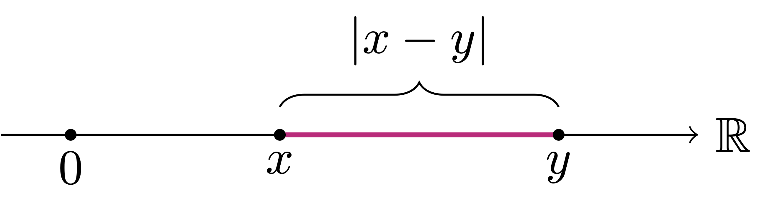
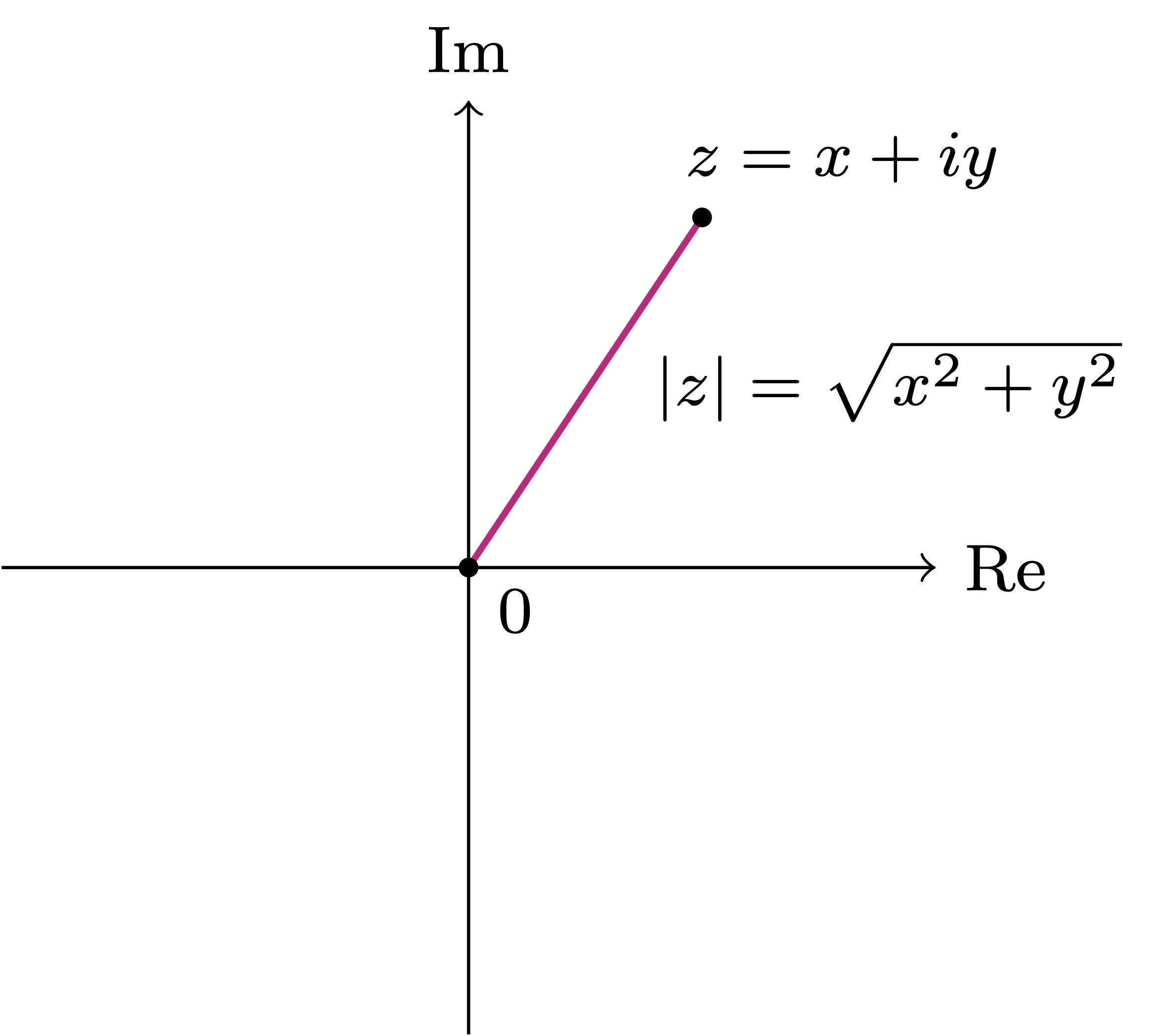
The Cartesian representation allows us to introduce a distance between two complex numbers. Let us start with the distance between a complex number $z=x+iy$ and $0$. By Pythagoras Theorem this distance is given by $$\sqrt{x^2+y^2},$$ see Figure 5.2. We give a name to this quantity.

Definition 21: Modulus

The modulus of a complex number $z=x+iy$ is defined by $$|z|:=\sqrt{x^2+y^2}.$$

Note that the distance between $z$ and $0$ is always a non-negative number.

Remark 22: Modulus of Real numbers

A real number $x\in \mathbb{R}$ can be written as $$x=x+0i\in \mathbb{C}.$$ Hence the modulus of $x$ is given by $$|x|=\sqrt{x^2+0^2}=\sqrt{x^2}.$$ The above coincides with the absolute value of $x$. This explains why the notation for modulus in $\mathbb{C}$ is the same as the one for absolute value in $\mathbb{R}$.

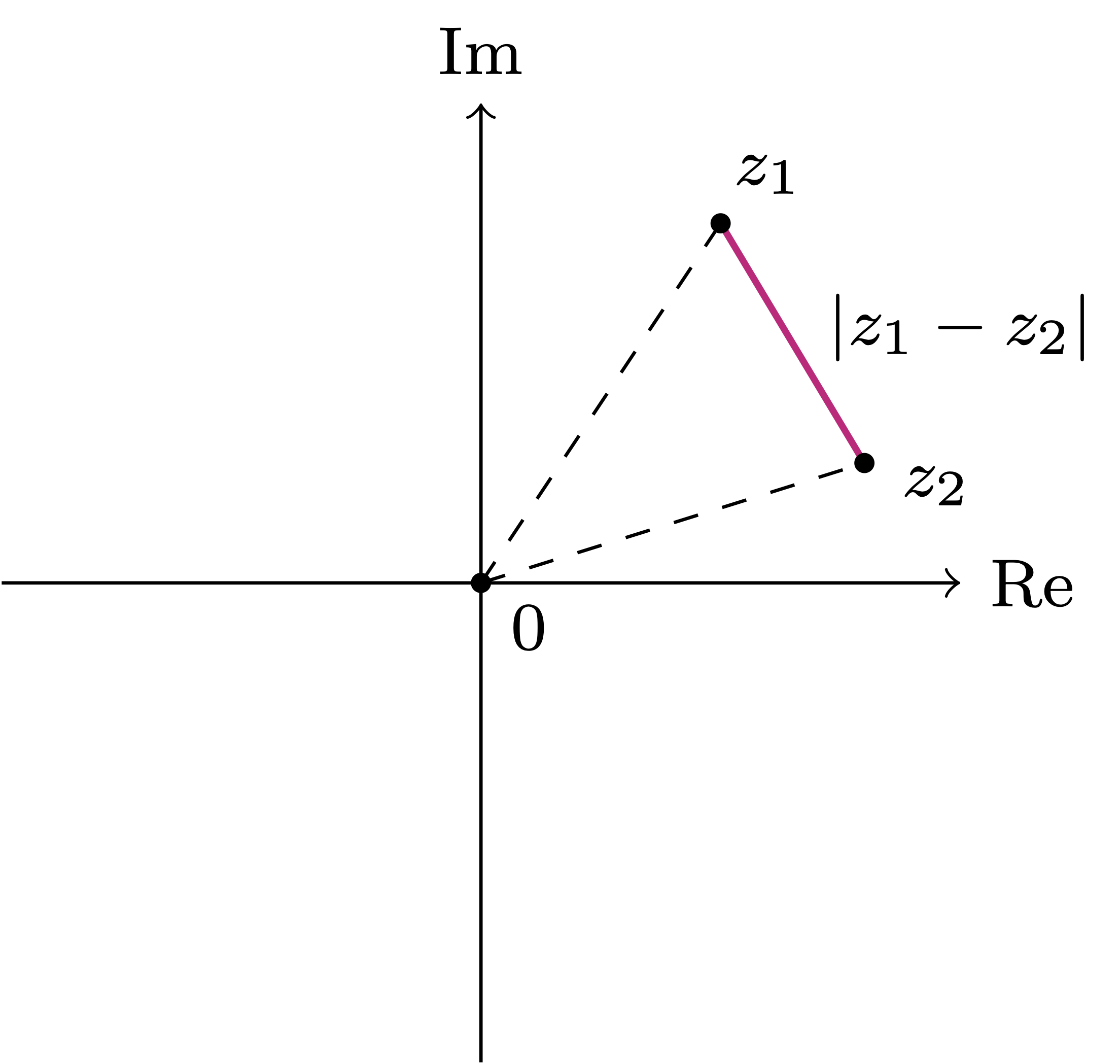
We can now define the distance between two complex numbers.

Definition 23: Distance in $\mathbb{C}$

Given $z_1,z_2\in \mathbb{C}$, we define the distance between $z_1$ and $z_2$ as the quantity $$|z_1-z_2|.$$

The geometric intuition of why the quantity $|z_1-z_2|$ is defined as the distance between $z_1$ and $z_2$ is given in Figure 5.3.

Figure 5.3: The difference $z_1-z_2$ of the two points $z_1,z_2\in \mathbb{C}$ is given by the magenta vector. We define $|z_1-z_2|$ as the distance between $z_1$ and $z_2$.

Theorem 24

Given $z_1,z_2\in \mathbb{C}$, we have $$|z_1-z_2|=\sqrt{(x_1-x_2{)}^2+(y_1-y_2{)}^2}.$$

Proof

We have $$z_1-z_2=(x_1-x_2)+i(y_1-y_2).$$ Therefore, by definition of modulus, $$|z_1-z_2|=\sqrt{(x_1-x_2{)}^2+(y_1-y_2{)}^2}.$$

Example 25

Question. Compute the distance between $$z=2-4i,w=-5+i.$$

Solution. The distance is $$\begin{array}{rl}|z-w|& =|(2-4i)-(-5+i)|\\ & =|7-5i|\\ & =\sqrt{7^2+(-5{)}^2}\\ & =\sqrt{74}\end{array}$$

5.3.2 Properties of modulus

The modulus has the following properties.

Theorem 26

Let $z,z_1,z_2\in \mathbb{C}$. Then

1. $|z_1\cdot z_2|=\left|z_1\right|\left|z_2\right|$

2. $\left|z^n\right|=|z{|}^n$ for all $n\in \mathbb{N}$

3. $z\cdot \overline{z}=|z{|}^2$

Proof

Part 1. We have $$\begin{array}{rl}{z}_1\cdot z_2& =(x_1+i{y}_1)\cdot (x_2+i{y}_2)\\ & =(x_1{x}_2-y_1{y}_2)+i(x_2{y}_1+x_1{y}_2)\end{array}$$ and therefore $$\begin{array}{rl}|z_1\cdot z_2|& =\sqrt{(x_1{x}_2-y_1{y}_2{)}^2+(x_2{y}_1+x_1{y}_2{)}^2}\\ & =\sqrt{x_1^2{x}_2^2+y_1^2{y}_2^2+x_2^2{y}_1^2+x_1^2{y}_2^2}.\end{array}$$ On the other hand, $$|z_1|=\sqrt{x_1^2+y_1^2},|z_2|=\sqrt{x_2^2+y_2^2}$$ so that $$\begin{array}{rl}|z_1||z_2|& =\sqrt{x_1^2+y_1^2}\sqrt{x_2^2+y_2^2}\\ & =\sqrt{x_1^2{x}_2^2+y_1^2{y}_2^2+x_2^2{y}_1^2+x_1^2{y}_2^2}\end{array}$$ proving that $|z_1\cdot z_2|=\left|z_1\right|\left|z_2\right|$.

Part 2. Exercise. It easily follows from Point 1 and induction.

Part 3. Let $z=x+iy$ for some $x,y\in \mathbb{R}$. Then,

$$\begin{array}{rl}z\cdot \overline{z}& =(x+iy)(x-iy)\\ & =x^2-(iy{)}^2\\ & =x^2+y^2\\ & =|z{|}^2\end{array}$$

The modulus in $\mathbb{C}$ satisfies the triangle inequality.

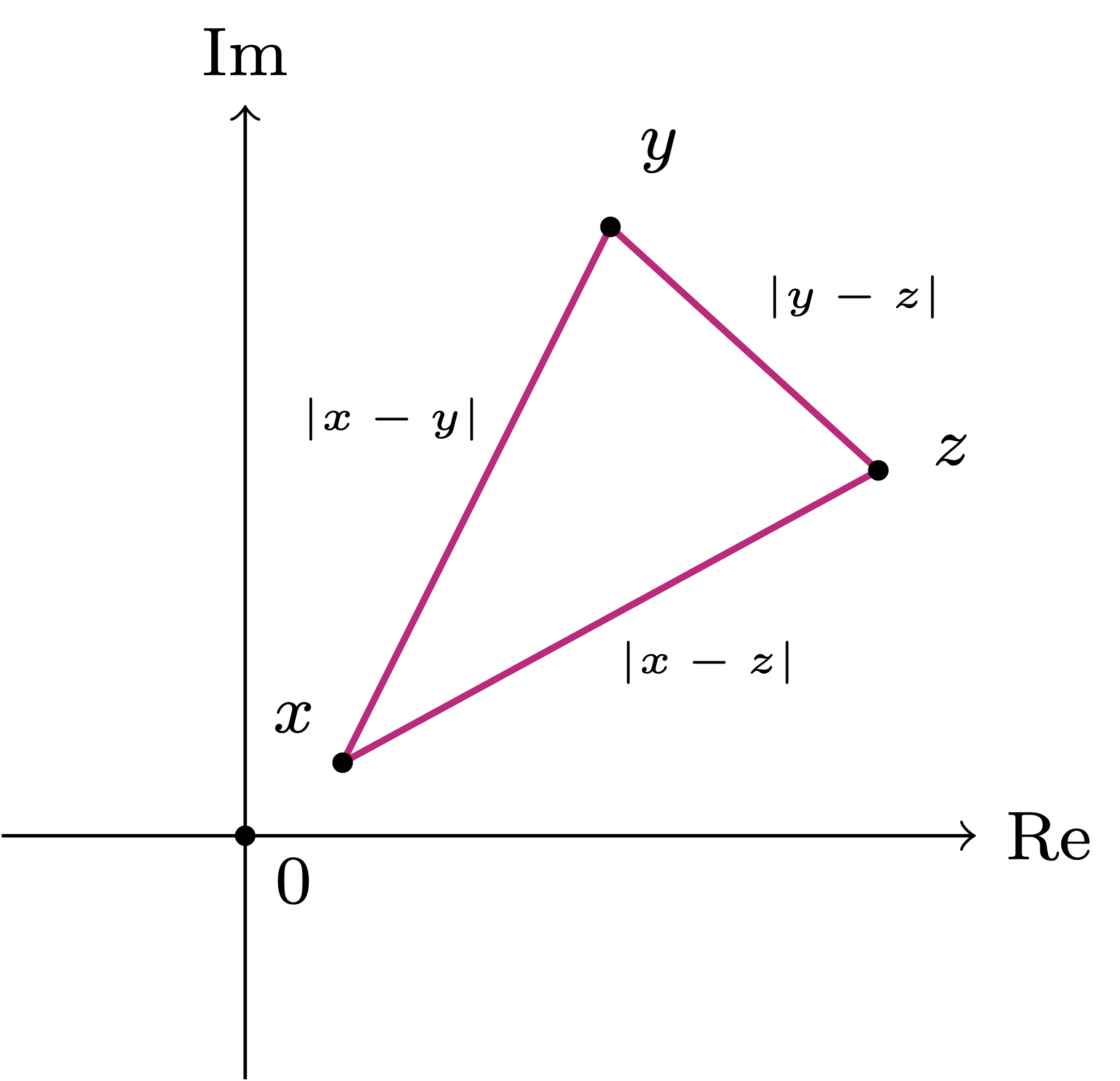
Theorem 27: Triangle inequality in $\mathbb{C}$

For all $x,y,z\in \mathbb{C}$,

1. $|x+y|\le |x|+|y|$

2. $|x-z|\le |x-y|+|y-z|$

Proof

Part 1. Suppose that $x=a+ib$ and $y=c+id$ for $a,b,c,d\in \mathbb{R}$. Then, $$|x+y|=|(a+c)+i(b+d)|=\sqrt{(a+c{)}^2+(b+d{)}^2}.$$ Therefore the inequality $$\begin{array}{}\text{(5.2)}& |x+y|\le |x|+|y|\end{array}$$ is equivalent to $$\begin{array}{}\text{(5.3)}& \sqrt{(a+c{)}^2+(b+d{)}^2}\le \sqrt{a^2+b^2}+\sqrt{c^2+d^2}.\end{array}$$ Now note that, for $A,B\in \mathbb{R}$, we have that $$\begin{array}{}\text{(5.4)}& A^2\le B^2⟹|A|\le |B|.\end{array}$$ In the two reverse implications $⟸$ below we will use (5.4): $$\begin{array}{rl}& \sqrt{(a+c{)}^2+(b+d{)}^2}\le \sqrt{a^2+b^2}+\sqrt{c^2+d^2}\\ ⟸& (a+c{)}^2+(b+d{)}^2\le {(\sqrt{a^2+b^2}+\sqrt{c^2+d^2})}^2\\ ⟺& a^2+2ac+c^2+b^2+2bd+d^2\le a^2+b^2+2\sqrt{a^2+b^2}\sqrt{c^2+d^2}+c^2+d^2\\ ⟺& ac+bd\le \sqrt{a^2+b^2}\sqrt{c^2+d^2}\\ ⟸& (ac+bd{)}^2\le (a^2+b^2)(c^2+d^2)\\ ⟺& a^2{c}^2+2abcd+b^2{d}^2\le a^2{c}^2+a^2{d}^2+b^2{c}^2+b^2{d}^2\\ ⟺& a^2{d}^2+b^2{c}^2-2abcd\ge 0\\ ⟺& (ad-bc{)}^2\ge 0.\end{array}$$

This last statement is clearly true, since $ad-bc\in \mathbb{R}$. Therefore (5.3) holds, and so (5.2) follows.

Part 2. Using (5.2) we estimate $$|x-z|=|x-y+y-z|\le |x-y|+|y-z|.$$

Remark 28: Geometric interpretation of triangle inequality

We finally have a justification of why the inequality $$|x-z|\le |x-y|+|y-z|$$ is called triangle inequality: By drawing three points $x,y,z\in \mathbb{C}$ in the complex plane, the distance between $x$ and $z$ is shorter than the distance to go from $x$ to $z$ via the point $y$, see Figure 5.4.

Figure 5.4: Let $x,y,z\in \mathbb{C}$. The distance between $x$ and $z$ is shorter than the distance to go from $x$ to $z$ via the point $y$.

5.4 Polar coordinates

We have seen that we can identify a complex number $z=x+iy$ by a point in the complex plane with Cartesian coordinates $(x,y)$. We can also specify the point $(x,y)$ by using the so-called polar coordinates $(\rho ,\theta )$, where

• $\rho$ is the distance between $z$ and the origin $$\rho =|z|=\sqrt{x^2+y^2}$$

• $\theta$ is the angle between the line connecting the origin and $z$ and the positive real axis, see Figure 5.5.

Figure 5.5: Polar coordinates $(\rho ,\theta )$ for the complex number $z\in \mathbb{C}$.

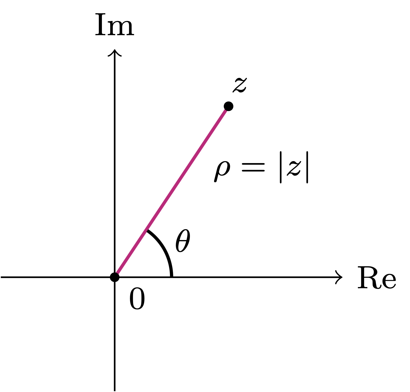
We give such angle a name.

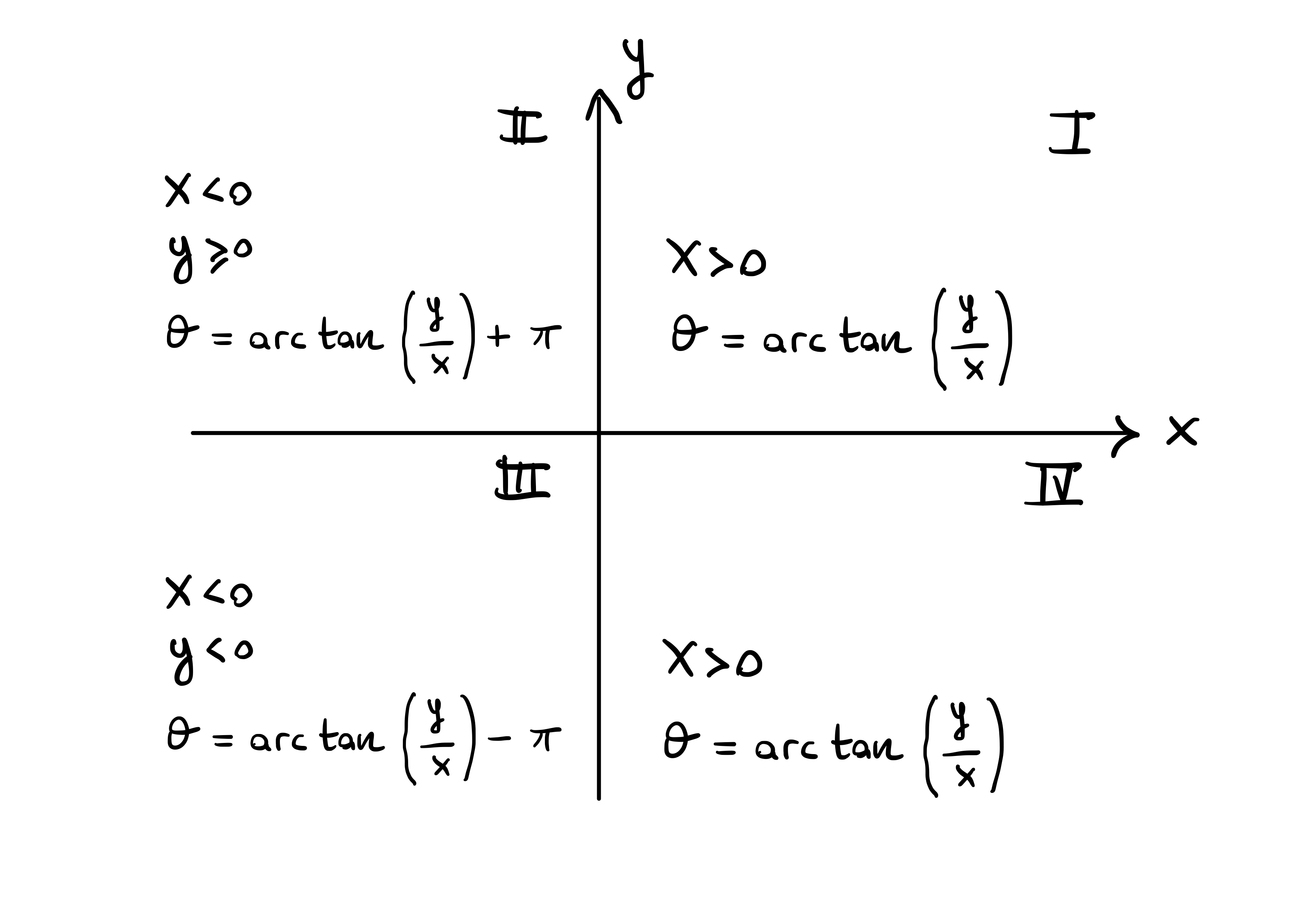
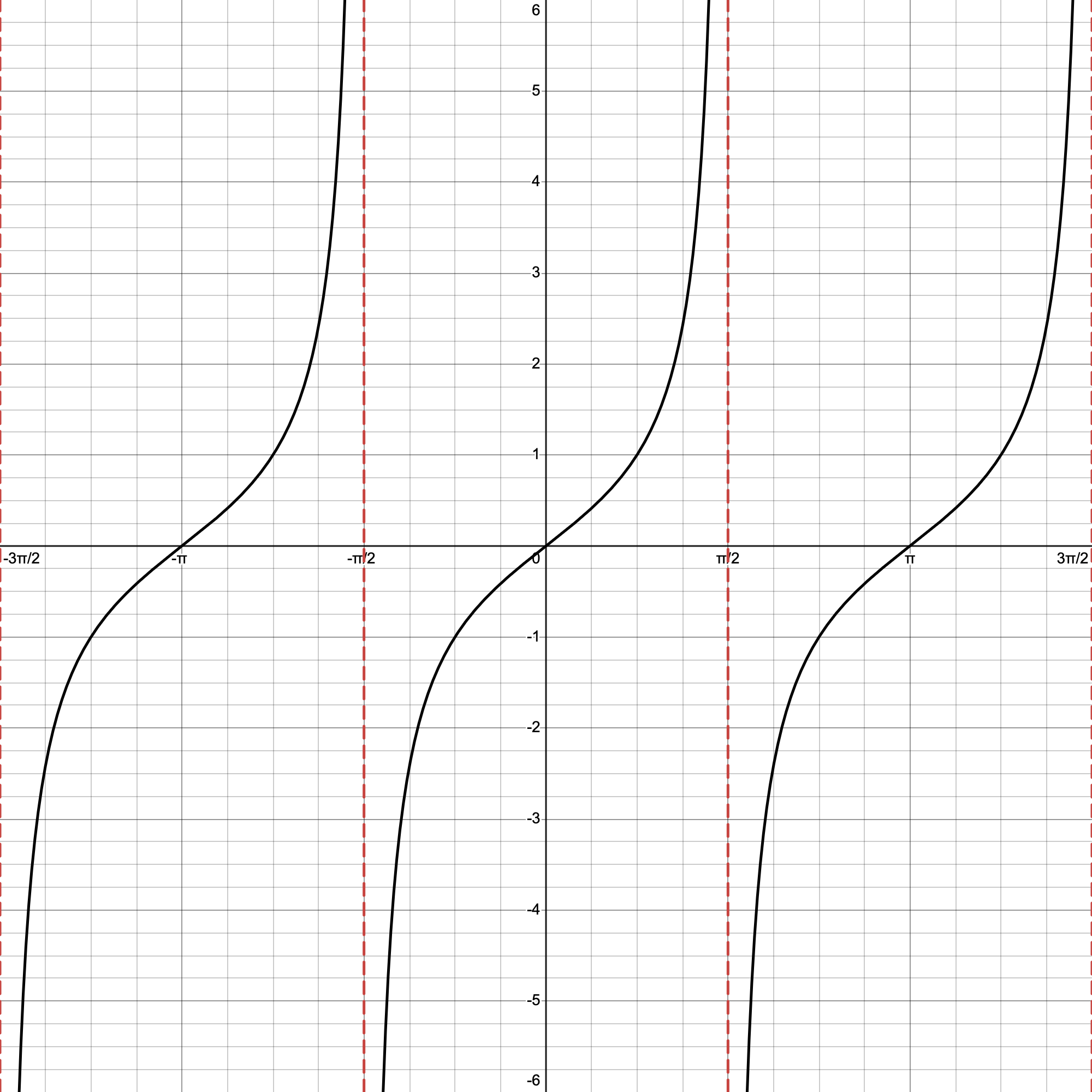
Definition 29: Argument

Let $z\in \mathbb{C}$. The angle $\theta$ between the line connecting the origin and $z$ and the positive real axis is called the argument of $z$, and is denoted by $$\theta :=\arg (z).$$

Warning

We always use angles in radians, not degrees. Make sure your calculator is set to radians if you want to use it to compute angles.

Remark 30: Principal Value

The argument of a complex number is not uniquely defined. We can always add an integer number of times $2\pi$ to the argument to specify the same point. We usually use the convention to choose the argument in the interval $(-\pi ,\pi ]$. This is called the principal value of the argument function. Therefore the complex numbers in the upper half plane have a positive argument, and the ones in the lower half plane have a negative argument.

Example 31

We have the following arguments: $$\begin{array}{rlrl}& \arg (1)=0& & \arg (i)=\frac{\pi }{2}\\ & \arg (-1)=\pi & & \arg (-i)=-\frac{\pi }{2}\\ & \arg (1+i)=\frac{1}{4}\pi & & \arg (-1-i)=-\frac{3}{4}\pi \end{array}$$

We can represent any non-zero complex number in polar coordinates.

Theorem 32: Polar coordinates

Let $z\in \mathbb{C}$ with $z=x+iy$ and $z\ne 0$. Then $$x=\rho \cos (\theta ),y=\rho \sin (\theta ),$$ where $$\rho :=|z|=\sqrt{x^2+y^2},\theta :=\arg (z).$$

The proof of Theorem 77 is trivial, and is based on basic trigonometry and definition of $\arg (z)$. Complex numbers in polar form can be useful. We give a name to such polar form.

Definition 33: Trigonometric form

Let $z\in \mathbb{C}$. The trigonometric form of $z$ is $$z=|z|[\cos (\theta )+i\sin (\theta )],$$ where $\theta =\arg (z)$.

Example 34

Question. Suppose that $z\in \mathbb{C}$ has polar coordinates $$\rho =\sqrt{8},\theta =\frac{3}{4}\pi .$$ Therefore, the trigonometric form of $z$ is $$z=\sqrt{8}[\cos \left(\frac{3}{4}\pi \right)+i\sin \left(\frac{3}{4}\pi \right)].$$ Write $z$ in cartesian form.

Solution. We have $$\begin{array}{c}x=\rho \cos (\theta )=\sqrt{8}\cos \left(\frac{3}{4}\pi \right)=-\sqrt{8}\cdot \frac{\sqrt{2}}{2}=-2\\ y=\rho \sin (\theta )=\sqrt{8}\sin \left(\frac{3}{4}\pi \right)=\sqrt{8}\cdot \frac{\sqrt{2}}{2}=2.\end{array}$$ Therefore, the cartesian form of $z$ is $$z=x+iy=-2+2i.$$

As a consequence of Theorem 77 we obtain a formula for computing the argument.

Corollary 35: Computing $\arg (z)$

Let $z\in \mathbb{C}$ with $z=x+iy$ and $z\ne 0$. Then $$\arg (z)=\{\begin{array}{ll}\arctan \left({\displaystyle \frac{y}{x}}\right)& \text{ if }x>0\\ \arctan \left({\displaystyle \frac{y}{x}}\right)+\pi & \text{ if }x<0\text{and}y\ge 0\\ \arctan \left({\displaystyle \frac{y}{x}}\right)-\pi & \text{ if }x<0\text{and}y<0\\ {\displaystyle \frac{\pi }{2}}& \text{ if }x=0\text{and}y>0\\ -{\displaystyle \frac{\pi }{2}}& \text{ if }x=0\text{and}y<0\end{array}$$ where $\arctan$ is the inverse of $\tan$.

Proof

Using the polar coordinates formulas from Theorem 77, we get $$\frac{y}{x}=\frac{\rho \sin (\theta )}{\rho \cos (\theta )}=\tan (\theta ).$$ The thesis can be obtained by carefully inverting the tangent: With reference to Figure 5.6 and Figure 5.7, we have:

1. When $x>0$: Then $z=x+iy$ belongs to the 1st or 4th quadrant. Therefore the argument of $z$ is $\theta \in (-\pi /2,\pi /2)$. Such interval coincides with the domain of $\tan$, and therefore $$\theta =\arctan \left({\displaystyle \frac{y}{x}}\right).$$

2. When $x<0$ and $y\ge 0$: Then $z=x+iy$ lies in the 2nd quadrant. Thus, the argument of $z$ is $\theta \in (\pi /2,\pi )$. Hence $$\theta =\arctan \left({\displaystyle \frac{y}{x}}\right)+\pi .$$

3. When $x<0$ and $y<0$: Then $z=x+iy$ lies in the 3rd quadrant. Thus, the argument of $z$ is $\theta \in (-\pi ,\pi /2)$. Hence $$\theta =\arctan \left({\displaystyle \frac{y}{x}}\right)-\pi .$$

4. When $x=0$ and $y>0$: Then $z=iy$ is imaginary with $y>0$, meaning that $\theta =\pi /2$.

5. When $x=0$ and $y<0$: Then $z=iy$ is imaginary with $y<0$, meaning that $\theta =-\pi /2$.

This exhausts all the cases, and the proof is concluded.

Figure 5.6: The definition of $\arg (z)$ depends on the position of $z$ in the complex plane.

Figure 5.7: Plot of the tangent function for $\theta$ between $-\frac{3\pi }{2}$ and $\frac{3\pi }{2}$.

Example 36

Question. Compute the arguments of the complex numbers $$z=3+4i,\overline{z}=3-4i,-\overline{z}=-3+4i,-z=-3-4i.$$

Solution. Using the formula for $\arg$ in Corollary 98 we have $$\begin{array}{rl}\arg (3+4i)& =\arctan \left(\frac{4}{3}\right)\\ \arg (3-4i)& =\arctan (-\frac{4}{3})=-\arctan \left(\frac{4}{3}\right)\\ \arg (-3+4i)& =\arctan (-\frac{4}{3})+\pi =-\arctan \left(\frac{4}{3}\right)+\pi \\ \arg (-3-4i)& =\arctan \left(\frac{4}{3}\right)-\pi \end{array}$$

5.5 Exponential form

We have seen that we can represent complex numbers in

• Cartesian form
• Trigonometric form

We now introduce a third way of representing complex numbers: the exponential form. For this, we need Euler’s identity:

Theorem 37: Euler’s identity

For all $\theta \in \mathbb{R}$ it holds $$e^{i\theta }=\cos (\theta )+i\sin (\theta ).$$

Proof

The proof of this theorem uses complex power series. We have not yet introduced series. However, we carry out the proof formally, assuming that all the quantities below converge. We have the following Taylor series at $x_0=0$ (you might know them from calculus): $$\begin{array}{rl}{e}^x& =1+x+\frac{x^2}{2!}+\frac{x^3}{3!}+\frac{x^4}{4!}+\frac{x^5}{5!}+\frac{x^6}{6!}+\frac{x^7}{7!}+\dots \\ \sin (x)& =\frac{x}{1!}-\frac{x^3}{3!}+\frac{x^5}{5!}-\frac{x^7}{7!}+\dots \\ \cos (x)& =1-\frac{x^2}{2!}+\frac{x^4}{4!}-\frac{x^6}{6!}+\dots \end{array}$$ The above identities also hold for $x\in \mathbb{C}$. Hence we can substitute $x=i\theta$ in the series for $e^x$ to obtain $$\begin{array}{rl}{e}^{i\theta }& =1+i\theta +\frac{(i\theta {)}^2}{2!}+\frac{(i\theta {)}^3}{3!}+\frac{(i\theta {)}^4}{4!}+\frac{(i\theta {)}^5}{5!}+\frac{(i\theta {)}^6}{6!}+\frac{(i\theta {)}^7}{7!}\dots \\ & =1+i\theta -\frac{{\theta }^2}{2!}-i\frac{{\theta }^3}{3!}+\frac{{\theta }^4}{4!}+i\frac{{\theta }^5}{5!}-\frac{{\theta }^6}{6!}-i\frac{{\theta }^7}{7!}+\dots \\ & =\cos (\theta )+i\sin (\theta ),\end{array}$$ where in the second equality we used that $i^2=-1$, and where the third equality follows by observing that all terms with an even power of $\theta$ are exactly the terms in the expansion of $\cos (\theta )$, and all terms with an odd power of $\theta$ are exactly the terms in the expansion of $\sin (\theta )$ multiplied by $i$.

Theorem 38

For all $\theta \in \mathbb{R}$ it holds $$\left|e^{i\theta }\right|=1.$$

Proof

From Euler’s identity in Theorem 100 we get $$\left|e^{i\theta }\right|=|\cos (\theta )+i\sin (\theta )|=\sqrt{{\cos }^2(\theta )+{\sin }^2(\theta )}=1.$$

Theorem 39

Let $z\in \mathbb{C}$ with $z=x+iy$ and $z\ne 0$. Then $$z=\rho e^{i\theta },$$ where $$\rho :=|z|=\sqrt{x^2+y^2},\theta :=\arg (z).$$

Proof

By Theorem 77 we have $$x=\rho \cos (\theta ),y=\rho \sin (\theta ).$$ Hence $$\begin{array}{rl}z& =x+iy\\ & =\rho \cos (\theta )+i\rho \sin (\theta )\\ & =\rho e^{i\theta },\end{array}$$ where in the last line we used Euler’s identity in Theorem 100.

Definition 40: Exponential form

The exponential form of a complex number $z\in \mathbb{C}$ is $$z=\rho e^{i\theta }=|z|e^{i\arg (z)}.$$

Example 41

Question. Write the number $$z=-2+2i$$ in exponential form.

Solution. From Example 97 we know that $z=-2+2i$ can be written in trigonometric form as $$z=\sqrt{8}[\cos \left(\frac{3}{4}\pi \right)+i\sin \left(\frac{3}{4}\pi \right)].$$ By Euler’s identity we hence obtain the exponential form $$z=\sqrt{8}{e}^{i\frac{3}{4}\pi }.$$

Remark 42: Periodicity of exponential

For all $k\in \mathbb{Z}$ we have $$\begin{array}{}\text{(5.5)}& e^{i\theta }=e^{i(\theta +2\pi k)},\end{array}$$ meaning that the complex exponential is $2\pi$-periodic. As we did for the principal value of the argument, we select $\theta$ in (5.5) so that $\theta \in (-\pi ,\pi ]$.

Proof

Equation (5.5) follows immediately by Euler’s identity and periodicity of $\cos$ and $\sin$, since $$\begin{array}{rl}{e}^{i(\theta +2\pi k)}& =\cos (\theta +2\pi k)+i\sin (\theta +2\pi k)\\ & =\cos (\theta )+i\sin (\theta )=e^{i\theta }.\end{array}$$

The exponential form is very useful for computing products and powers of complex numbers.

Proposition 43

Let $z,z_1,z_2\in \mathbb{C}$ and suppose that $$z=\rho e^{i\theta },z_1={\rho }_1{e}^{i{\theta }_1},z_2={\rho }_2{e}^{i{\theta }_2}.$$ We have $$z_1\cdot z_2={\rho }_1{\rho }_2{e}^{i({\theta }_1+{\theta }_2)},z^n={\rho }^n{e}^{in\theta },$$ for all $n\in \mathbb{N}$.

The proof follows immediately by the properties of the exponential. Let us see some applications of Propostion 106.

Example 44

Question. Compute $(-2+2i{)}^4$.

Solution. We have two possibilities:

1. Use the binomial theorem: $$\begin{array}{rl}(-2+2i{)}^4& =(-2{)}^4+\left(\begin{array}{c}4\\ 1\end{array}\right)(-2{)}^3\cdot 2i+\left(\begin{array}{c}4\\ 2\end{array}\right)(-2{)}^2\cdot (2i{)}^2\\ & +\left(\begin{array}{c}4\\ 3\end{array}\right)(-2)\cdot (2i{)}^3+(2i{)}^4\\ & =16-4\cdot 8\cdot 2i-6\cdot 4\cdot 4+4\cdot 2\cdot 8i+16\\ & =16-64i-96+64i+16=-64.\end{array}$$

2. A much simpler calculation is possible by using the exponential form: We know that $$-2+2i=\sqrt{8}{e}^{i\frac{3}{4}\pi }$$ by Example 104. Hence $$(-2+2i{)}^4={\left(\sqrt{8}{e}^{i\frac{3}{4}\pi }\right)}^4=8^2{e}^{i3\pi }=-64,$$ where we used that $$e^{i3\pi }=e^{i\pi }=\cos (\pi )+i\sin (\pi )=-1$$ by $2\pi$ periodicity of $e^{i\theta }$ and Euler’s identity.

Definition 45: Complex exponential

The complex exponential of $z=a+ib\in \mathbb{C}$ is defined as $$e^z=e^a{e}^{ib}.$$

The complex exponential behaves exactly as exponentials should.

Theorem 46

Let $z,w\in \mathbb{C}$. Then $$\begin{array}{}\text{(5.6)}& e^{z+w}=e^z{e}^w,(e^z{)}^w=e^{zw}.\end{array}$$

We still do not have the technical means to prove this Theorem. The idea is to express $e^z$ as $$\begin{array}{}\text{(5.7)}& e^z=\sum _{k=0}^{\mathrm{\infty }}\frac{z^n}{n!},\end{array}$$ where the convergence is intendend in the sense of complex series. The properties at (5.6) then follow from manipulating the series on the RHS of (5.7).

Example 47

Question. Compute $i^i$.

Solution. We know that $$|i|=1,\arg (i)=\frac{\pi }{2}.$$ Hence we can write $i$ in exponential form $$i=|i|e^{i\arg (i)}=e^{i\frac{\pi }{2}}.$$ Therefore $$i^i={\left(e^{i\frac{\pi }{2}}\right)}^i=e^{i^2\frac{\pi }{2}}=e^{-\frac{\pi }{2}}.$$

5.6 Fundamental Theorem of Algebra

We started the introduction to complex numbers with the following question:

Question 48

Is there a number $x\in \mathbb{R}$ such that $$\begin{array}{}\text{(5.8)}& x^2=-1?\end{array}$$

The answer is no. For this reason we introduced the complex number $i$, which satisfies $$i^2=-1.$$ Therefore (5.8) has solution in $\mathbb{C}$, with $x=i$. Moreover, note that $$(-i{)}^2=(-1{)}^2{i}^2=-1.$$ Hence (5.8) has two solutions in $\mathbb{C}$, given by $$x_1=i,x_2=-i.$$

It turns out that the set $\mathbb{C}$ is so large, that not only we are able to solve (5.8), but in fact any polynomial equation.

Theorem 49: Fundamental theorem of algebra

Let $p_n(z)$ be a polynomial of degree $n$ with complex coefficients, i.e., $$p_n(z)=a_n{z}^n+a_{n-1}{z}^{n-1}+\dots +a_{1}z+a_0,$$ for some coefficients $a_n,\dots ,a_0\in \mathbb{C}$ with $a_n\ne 0$. There exist $$z_1,\dots ,z_n\in \mathbb{C}$$ solutions to the polynomial equation $$\begin{array}{}\text{(5.9)}& p_n(z)=a_n{z}^n+a_{n-1}{z}^{n-1}+\dots +a_{1}z+a_0=0.\end{array}$$ In particular, $p_n$ factorizes as $$\begin{array}{}\text{(5.10)}& p_n(z)=a_n(z-z_1)(z-z_2)\cdots (z-z_n).\end{array}$$

Theorem 111 says that equation (5.9) admits $n$ complex solutions:

• We call these solutions zeros, or also roots.
• We call the expression (5.10) a factorization of the polynomial $p_n$.

Several proofs of Theorem 111 exist in the literature, but they all use mathematical tools which are out of reach for now. Therefore we will not show a proof. For example one can prove Theorem 111 by

• Liouville’s theorem (complex analysis)
• Homotopy arguments (general topology)
• Fundamental Theorem of Galois Theory (algebra)

Example 50

Question. Find all the complex solutions to $$\begin{array}{}\text{(5.11)}& z^2=-1\end{array}$$

Solution. The equation $z^2=-1$ is equivalent to $$p(z)=0,p(z):=z^2+1.$$ Since $p$ has degree $n=2$, the Fundamental Theorem of Algebra tells us that there are two solutions to (5.11). We have already seen that these two solutions are $z=i$ and $z=-i$. Then $p$ factorizes as $$p(z)=z^2+1=(z-i)(z+i).$$

Example 51

Question. Find all the complex solutions to $$\begin{array}{}\text{(5.12)}& z^4-1=0.\end{array}$$

Solution The associated polynomial equation is $$p(z)=0,p(z):=z^4-1.$$ Since $p$ has degree $n=4$, the Fundamental Theorem of Algebra tells us that there are $4$ solutions to (5.12). Let us find such solutions. We use the well known identity $$a^2-b^2=(a+b)(a-b),\mathrm{\forall }a,b\in \mathbb{R},$$ to factorize $p$. We get: $$p(z)=(z^4-1)=(z^2+1)(z^2-1).$$ We know that $$z^2+1=0$$ has solutions $z=\pm i$. Instead
$$z^2-1=0$$ has solutions $x=\pm 1$. Hence, the four solutions of (5.12) are given by $$z=1,-1,i,-i,$$ and $p$ factorizes as $$p(z)=z^4-1=(z-1)(z+1)(z-i)(z+i).$$

Definition 52: Multiplicity

Suppose that the polynomial $p_n$ factorizes as $$p_n(z)=a_n(z-z_1{)}^{k_1}(z-z_2{)}^{k_2}\cdots (z-z_m{)}^{k_m}$$ with $a_n\ne 0$, $z_1,\dots ,z_m\in \mathbb{C}$ and $k_1,\dots ,k_m\in \mathbb{N}$, $k_i\ge 1$. In this case $p_n$ has degree $$n=k_1+\dots +k_m=\sum _{i=1}^m{k}_i.$$ Note that $z_i$ is solves the equation $$p_n(z)=0$$ exactly $k_i$ times. We call $k_i$ the multiplicity of the solution $z_i$.

Example 53

The equation $$(z-1)(z-2{)}^2(z+i{)}^3=0$$ has 6 solutions:

• $z=1$ with multiplicity $1$
• $z=2$ with multiplicity $2$
• $z=-i$ with multiplicity $3$

5.7 Solving polynomial equations

The non-factorized version of the polynomial $$\begin{array}{}\text{(5.13)}& p(z)=(z-1)(z-2{)}^2(z+i{)}^3\end{array}$$ from Example 115 is $$\begin{array}{}\text{(5.14)}& \begin{array}{rl}p(z)=& z^6-(5-3i)z^5+(5-15i)z^4\\ & +(11+23i)z^3-(24+7i)z^2+(12-8i)z+4i\end{array}\end{array}$$ Question: How do we figure out the factorization at (5.13) if we are given $p$ in the form at (5.13)? More in general, consider the following question:

Question 54

The Fundamental Theorem of Algebra states that $$\begin{array}{}\text{(5.15)}& p_n(z)=0\end{array}$$ has $n$ complex solutions. How do we find such solutions in practice?

Answer: There is no general formula to solve (5.15) when $n\ge 5$. This is the content of the Abel-Ruffini Theorem.

Theorem 55: Abel-Ruffini

There is no elementary solution formula to the polynomial equation $$p_n(z)=0,$$ with $p_n$ polynomial of degree $n$, with $n\ge 5$.

Similarly to the Fundamental Theorem of Algebra, the proof of the Abel-Ruffini Theorem is out of reach for now. A proof can be carried out, for example, using Galois Theory.

There are however explicit formulas for solving (5.15) when $p_n$ has degree $n=2,3,4$.

5.7.1 Quadratic polynomials

Consider polynomial equations of order $n=2$, that is, equations of the form $$\begin{array}{}\text{(5.16)}& a{z}^2+bz+c=0.\end{array}$$ When the coefficients $a,b,c$ are real, the solutions are given by the well-known quadratic formula.

Proposition 56: Quadratic formula

Let $a,b,c\in \mathbb{R},a\ne 0$ and consider the equation at (5.16). Define $$\mathrm{\Delta }:=b^2-4ac\in \mathbb{R}.$$ The following hold:

1. If $\mathrm{\Delta }>0$ then (5.16) has two distinct real solutions $z_1,z_2\in \mathbb{R}$ given by $$z_1=\frac{-b-\sqrt{\mathrm{\Delta }}}{2a},z_2=\frac{-b+\sqrt{\mathrm{\Delta }}}{2a}.$$
2. If $\mathrm{\Delta }=0$ then (5.16) has one real solution $z\in \mathbb{R}$ with multiplicity $2$. Such solution is given by $$z=z_1=z_2=\frac{-b}{2a}.$$
3. If $\mathrm{\Delta }<0$ then (5.16) has two distinct complex solutions $z_1,z_2\in \mathbb{C}$ given by $$z_1=\frac{-b-i\sqrt{-\mathrm{\Delta }}}{2a},z_2=\frac{-b+i\sqrt{-\mathrm{\Delta }}}{2a},$$ where $\sqrt{-\mathrm{\Delta }}\in \mathbb{R}$, since $-\mathrm{\Delta }>0$.

In all cases, the polynomial at (5.16) factorizes as $$a{z}^2+bz+c=a(z-z_1)(z-z_2).$$

Example 57

Question. Solve the following equations:

1. $3z^2-6z+2=0$
2. $4z^2-8z+4=0$
3. $z^2+2z+3=0$

Solution.

1. We have that $$\mathrm{\Delta }=(-6{)}^2-4\cdot 3\cdot 2=12>0$$ Therefore the equation has two distinct real solutions, given by $$z=\frac{-(-6)\pm \sqrt{12}}{2\cdot 3}=\frac{6\pm \sqrt{12}}{6}=1\pm \frac{\sqrt{3}}{3}$$ In particular we have the factorization $$3z^2-6z+2=3(z-1-\frac{\sqrt{3}}{3})(z-1+\frac{\sqrt{3}}{3}).$$

2. We have that $$\mathrm{\Delta }=(-8{)}^2-4\cdot 4\cdot 4=0.$$ Therefore there exists one solution with multiplicity $2$. This is given by $$z=\frac{-(-8)}{2\cdot 4}=1.$$ In particular we have the factorization $$4z^2-8x+4=4(z-1{)}^2.$$

3. We have $$\mathrm{\Delta }=2^2-4\cdot 1\cdot 3=-8<0.$$ Therefore there are two complex solutions given by $$z=\frac{-2\pm i\sqrt{8}}{2\cdot 1}=-1\pm i\sqrt{2}.$$ In particular we have the factorization $$z^2+2z+3=(z+1-i\sqrt{2})(z+1+i\sqrt{2}).$$

So far we have considered the polynomial equation $$\begin{array}{}\text{(5.17)}& a{z}^2+bz+c=0,\end{array}$$ for $a,b,c\in \mathbb{R}$ and $a\ne 0$.

Question 58

What if $a,b,c\in \mathbb{C}$?

If $a,b,c\in \mathbb{C}$ then we might have $$\mathrm{\Delta }:=b^2-4ac\in \mathbb{C}.$$ Therefore it is not clear how to compute $$\sqrt{\mathrm{\Delta }}.$$ However, we can still use the quadratic equation to solve (5.17), as outlined in the next Proposition.

Proposition 59: Quadratic formula with complex coefficients

Let $a,b,c\in \mathbb{C},a\ne 0$. The two solutions to $$a{z}^2+bz+c=0$$ are given by $$z_1=\frac{-b+S_1}{2a},z_2=\frac{-b+S_2}{2a},$$ where $S_1$ and $S_2$ are the two solutions to $$z^2=\mathrm{\Delta },\mathrm{\Delta }:=b^2-4ac.$$

Remark 60

We want to check that the new formulas $$z_1=\frac{-b+S_1}{2a},z_2=\frac{-b+S_2}{2a},S_1^2=S_2^2=\mathrm{\Delta },$$ agree with the old formulas given in Proposition 116, when $a,b,c\in \mathbb{R}$.

To this end, note that $$\mathrm{\Delta }\in \mathbb{R},$$ when $a,b,c\in \mathbb{R}$. In this case the equation $$z^2=\mathrm{\Delta }$$ has the following solutions:

• If $\mathrm{\Delta }>0$ there are two real solutions $$S_1=-\sqrt{\mathrm{\Delta }},S_2=\sqrt{\mathrm{\Delta }}.$$
• If $\mathrm{\Delta }=0$ then $0$ is the only solution with multiplicity $2$. Hence $$S_1=S_2=0.$$
• If $\mathrm{\Delta }<0$, there are two complex solutions $$S_1=-i\sqrt{-\mathrm{\Delta }},S_2=i\sqrt{-\mathrm{\Delta }}.$$

Therefore the solutions $$z_1=\frac{-b+S_1}{2a},z_2=\frac{-b+S_2}{2a},$$ given in Proposition 116 coincide with the ones given in Proposition 118.

Example 61

Question Find all the solutions to $$\begin{array}{}\text{(5.18)}& \frac{1}{2}{z}^2-(3+i)z+(4-i)=0.\end{array}$$

Solution. We have $$\begin{array}{rl}\mathrm{\Delta }& =(-(3+i){)}^2-4\cdot \frac{1}{2}\cdot (4-i)\\ & =8+6i-8+2i\\ & =8i.\end{array}$$ Therefore $\mathrm{\Delta }\in \mathbb{C}$. We have to find solutions $S_1$ and $S_2$ to the equation $$\begin{array}{}\text{(5.19)}& z^2=\mathrm{\Delta }=8i.\end{array}$$ We look for solutions of the form $z=a+ib$. Then we must have that $$z^2=(a+ib{)}^2=a^2-b^2+2abi=8i.$$ Thus $$a^2-b^2=0,2ab=8.$$ From the first equation we conclude that $|a|=|b|$. From the second equation we have that $ab=4$, and therefore $a$ and $b$ must have the same sign. Hence $a=b$, and $$2ab=8⟹a=b=\pm 2.$$ From this we conclude that the solutions to (5.19) are $$S_1=2+2i,S_2=-2-2i.$$ Hence the solutions to (5.18) are $$\begin{array}{rl}{z}_1& =\frac{3+i+S_1}{2\cdot \frac{1}{2}}=3+i+S_1\\ & =3+i+2+2i=5+3i,\end{array}$$ and $$\begin{array}{rl}{z}_2& =\frac{3+i+S_2}{2\cdot \frac{1}{2}}=3+i+S_2\\ & =3+i-2-2i=1-i.\end{array}$$ In particular, the given polynomial factorizes as $$\begin{array}{rl}\frac{1}{2}{z}^2-(3+i)z+(4-i)& =\frac{1}{2}(z-z_1)(z-z_2)\\ & =\frac{1}{2}(z-5-3i)(z-1+i).\end{array}$$

In the above example it was a bit laborious to compute $S_1$ and $S_2$. In Section 5.8 and Section 5.9, we will explore a more general method to solve problems of the form $$z^n=\mathrm{\Delta }.$$

5.7.2 Higher order polynomials

Consider now polynomial equations $$p_n(z)=0,$$ with $p_n$ of degree $n=3,4$. Although general solution formulas exist for these cases, they are exceedingly lengthy, making them impractical for manual calculations. For example, Figure 5.8 shows the solution formula to the quartic equation $$z^4+a{z}^3+b{z}^2+cz+d=0,$$ when $a,b,c,d\in \mathbb{R}$.

Figure 5.8: Quartic formula to solve $z^4+a{z}^3+b{z}^2+cz+d=0$. Image from Wikipedia.

A more productive use of time is learning how to perform long polynomial division. A quick tutorial is available here: Polynomial_division.pdf.

Example 62

Question. Divide $6z^3+5z^2-7$ by $3z^2-2z-1$.

Solution. Using polynomial division, see Figure 5.9, we obtain $$6z^3+5z^2-7=(3z^2-2z-1)(2z+3)+(8z-4).$$

Figure 5.9: Example of polynomial long division between $6z^3+5z^2-7$ and $3z^2-2z-1$.

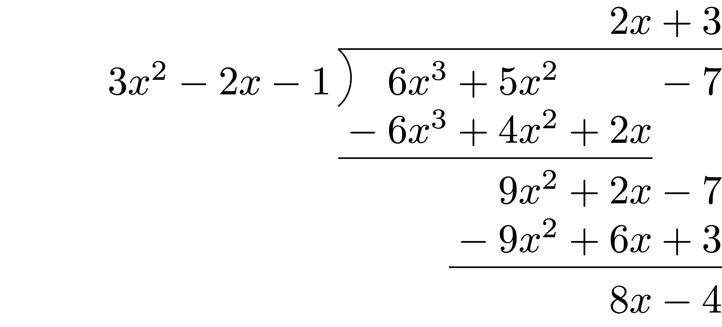
Sometimes, it is possible to solve equations of degree higher than 2, in case it is obvious from inspection that a certain number is a solution, e.g., when $z=-1,0,1$ is a solution.

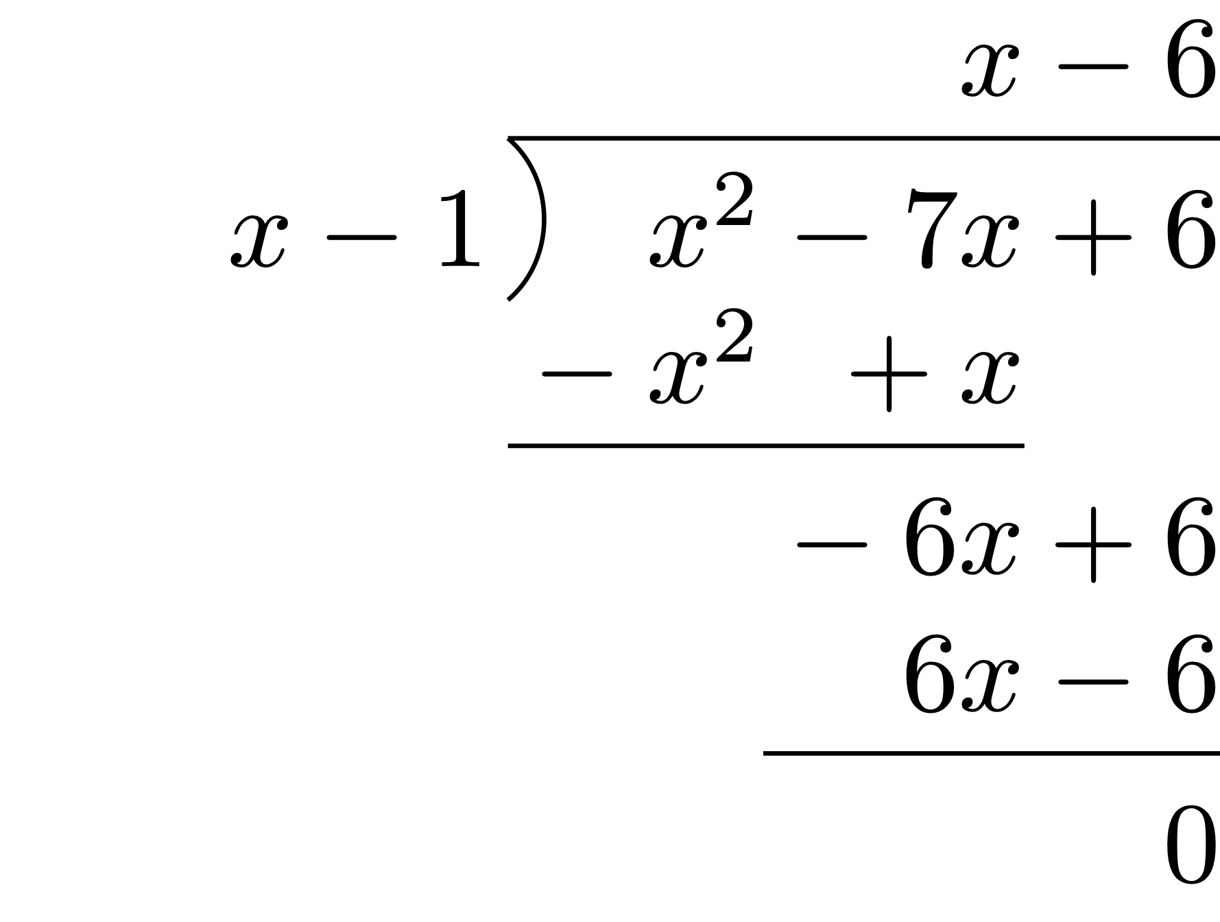
Example 63

Question. Consider the equation $$z^3-7z^2+6z=0.$$

1. Check whether $z=0,1,-1$ are solutions.
2. Using your answer from Point 1, and polynomial division, find all the solutions.

Solution.

1. By direct inspection we see that $z=0$ and $z=1$ are solutions.

2. Since $z=0$ is a solution, we can factorize $$z^3-7z^2+6z=z(z^2-7z+6).$$ We could now use the quadratic formula on the term $z^2-7z+6$ to find the remaining two roots. However, we have already observed that $z=1$ is a solution. Therefore $z-1$ divides $z^2-7z+6$. Using polynomial long division, see Figure 5.10, we find that $$\frac{z^2-7z+6}{z-1}=z-6.$$ Therefore the last solution is $z=6$, and $$z^3-7z^2+6z=z(z-1)(z-6).$$

Figure 5.10: Polynomial long division between $z^2-7z+6$ and $z-1$.

Example 64

Question. Find all the complex solutions to $$z^3-7z+6=0.$$

Solution. It is easy to see $z=1$ is a solution. This means that $z-1$ divides $z^3-7z+6$. By using polynomial long division, see Figure 5.11, we compute that $$\frac{z^3-7z+6}{z-1}=z^2+z-6.$$ We are now left to solve $$z^2+z-6=0.$$ Using the quadratic formula, we see that the above is solved by $z=2$ and $z=-3$. Therefore the given polynomial factorizes as $$z^3-7z+6=(z-1)(z-2)(z+3).$$

Figure 5.11: Polynomial long division between $z^3-7z+6$ and $z-1$.

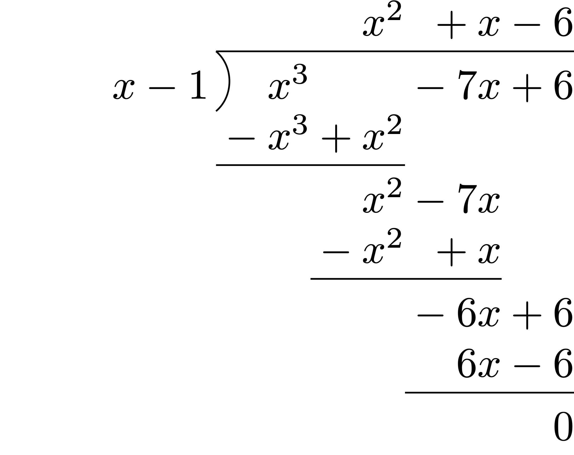
Example 65

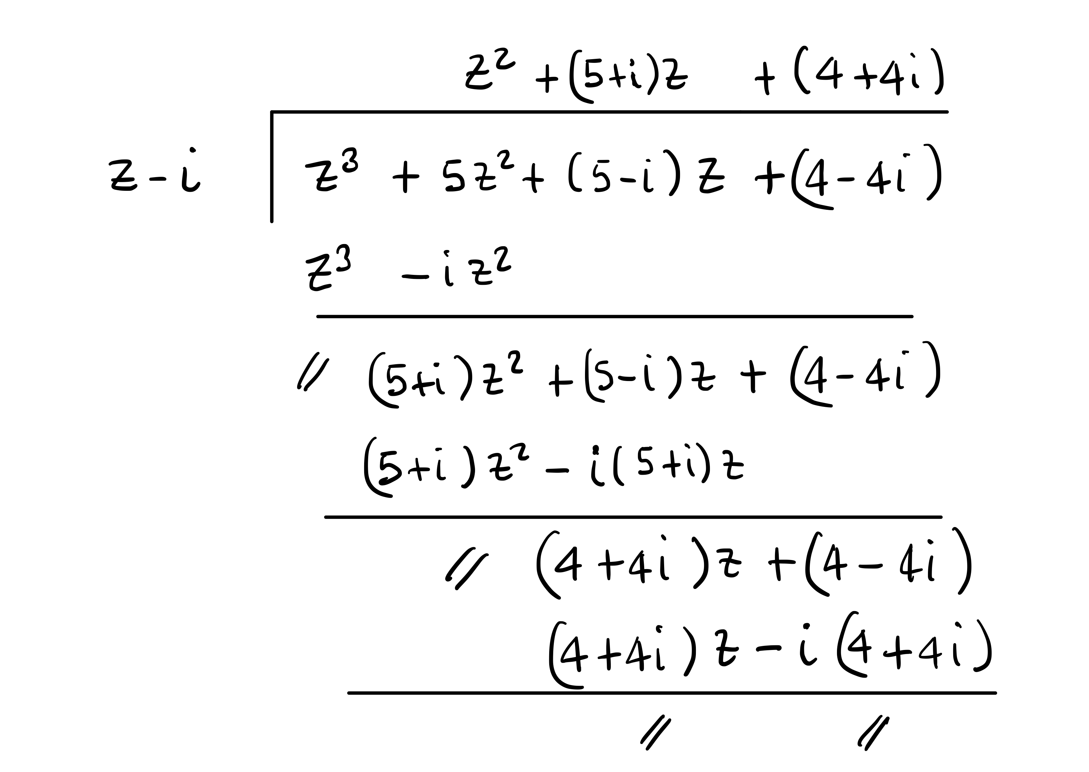
Question. Consider the equation $$z^3+5z^2+(5-i)z+(4-4i)=0.$$

1. Check whether $z=\pm i$ and $z=0,\pm 1$ are solutions.
2. By using polynomial division with complex coefficients, find all the solutions.

Solution.

1. By direct inspection, we see that $z=i$ is a solution.

2. Since $z=i$ is a solution, we know that $z-i$ divides $z^3+5z^2+(5-i)z+(4-4i)$. We now perform polynomial division by using the same method employed to divide polynomials with real coefficients: We just need to be mindful of the fact that coefficients are now complex, and thus, addition and multiplication have to be carried out in $\mathbb{C}$. Using polynomial long division, see Figure 5.12, we compute that $$z^3+5z^2+(5-i)z+(4-4i)=(z-i)(z^2+(5+i)z+(4-4i)).$$ We are now left to solve the second order equation $$z^2+(5+i)z+(4-4i)=0.$$ We compute that $$\mathrm{\Delta }=b^2-4ac=(5+1{)}^2-4(4-4i)=4(5+4i).$$ We now need to solve $$z^2=\mathrm{\Delta }.$$ We look for a solution in the form of $z=a+ib$. $$z^2=(a+ib{)}^2=a^2-b^2+2abi=8i.$$ Thus $$a^2-b^2=0,2ab=8.$$ From the first equation we conclude that $|a|=|b|$. From the second equation we have that $ab=4$, and therefore $a$ and $b$ must have the same sign. Hence $a=b$, and $$2ab=8⟹a=b=\pm 2.$$ From this we conclude that the solutions to (5.19) are $$S_1=2+2i,S_2=-2-2i.$$ Hence the solutions to (5.18) are $$\begin{array}{rl}{z}_1& =\frac{3+i+S_1}{2\cdot \frac{1}{2}}=3+i+S_1\\ & =3+i+2+2i=5+3i,\end{array}$$ and $$\begin{array}{rl}{z}_2& =\frac{3+i+S_2}{2\cdot \frac{1}{2}}=3+i+S_2\\ & =3+i-2-2i=1-i.\end{array}$$ In particular, the given polynomial factorizes as $$\begin{array}{rl}\frac{1}{2}{z}^2-(3+i)z+(4-i)& =\frac{1}{2}(z-z_1)(z-z_2)\\ & =\frac{1}{2}(z-5-3i)(z-1+i).\end{array}$$

Figure 5.12: Polynomial long division between $z^3+5z^2+(5-i)z+(4-4i)$ and $z-i$.

5.8 Roots of unity

Problem

Let $n\in \mathbb{N}$. We want to find all complex solutions to $$\begin{array}{}\text{(5.20)}& z^n=1.\end{array}$$

Note that $z=1$ is always a solution to (5.20) if $n$ is even. In such case also $z=-1$ is a solution. If we were only looking for solutions in $\mathbb{R}$, these two would be the only solutions.

However, the Fundamental Theorem of Algebra, see Theorem 111, tells us that there are $n$ complex solutions to (5.20).

Question 66

Is there a way to find all $n$ solutions?

Example 67

We have seen in Example 113 that the solutions to $$z^4=1$$ are $$z=-1,1,i,-i.$$ However, we could only compute these solutions thanks to the clever factorization $$z^4-1=(z^2+1)(z^2-1)=(z+i)(z-i)(z+1)(z-1).$$ It is not clear if and how this trick can be generalized to solve $$z^n=1$$ for arbitrary $n\in \mathbb{N}$.

The trick to find all $n$ solutions to (5.20) is to use the exponential form.

Theorem 68

Let $n\in \mathbb{N}$ and consider the equation $$\begin{array}{}\text{(5.21)}& z^n=1.\end{array}$$ All the $n$ solutions to (5.21) are given by $$z_k=\exp \left(i\frac{2\pi k}{n}\right),k=0,\dots ,n-1,$$ where $\exp (x)$ denotes $e^x$.

Proof

Rewrite $1$ in exponential form: $$1=|1|e^{i\arg (1)}=e^{i2\pi k},k\in \mathbb{Z}.$$ Therefore (5.21) is equivalent to $$z^n=e^{i2\pi k}.$$ By the properties of the exponential, we see that the above is solved by $$z_k=\exp \left(i\frac{2\pi k}{n}\right),k\in \mathbb{Z}.$$ By choosing $k=0,\dots ,n-1$ we obtain $n$ different solutions.

Definition 69

The $n$ solutions to $$z^n=1$$ are called the roots of unity.

Example 70

Question. Find all the solutions to $$z^4=1.$$

Solution. The $4$ solutions are given by $$z_k=\exp \left(i\frac{2\pi k}{4}\right)=\exp \left(i\frac{\pi k}{2}\right),$$ for $k=0,1,2,3$. We compute: $$\begin{array}{rlrl}{z}_0& =e^{i0}=1,& & z_1=e^{i\frac{\pi }{2}}=i,\\ z_2& =e^{i\pi }=-1,& & z_3=e^{i\frac{3\pi }{2}}=-i.\end{array}$$ Note that for $k=4$ we would again get the solution $z=e^{i2\pi }=1$.

Example 71

Question. Find all the solutions to $$z^3=1.$$

Solution. The $3$ solutions are given by $$z_k=\exp \left(i\frac{2\pi k}{3}\right),$$ for $k=0,1,2$. We compute: $$z_0=e^{i0}=1,z_1=e^{i\frac{2\pi }{3}},z_2=e^{i\frac{4\pi }{3}}.$$ We can write $z_1$ and $z_2$ in cartesian form: $$z_1=e^{i\frac{2\pi }{3}}=\cos \left(\frac{2\pi }{3}\right)+i\sin \left(\frac{2\pi }{3}\right)=-\frac{1}{2}+\frac{\sqrt{3}}{2}i$$ and $$z_2=e^{i\frac{4\pi }{3}}=\cos \left(\frac{4\pi }{3}\right)+i\sin \left(\frac{4\pi }{3}\right)=-\frac{1}{2}-\frac{\sqrt{3}}{2}i.$$

5.9 Roots in $\mathbb{C}$

Let $n\in \mathbb{N}$ and $c\in \mathbb{C}$. We want to give a meaning to $$\sqrt[n]{c}.$$ This means, we want to find all complex solutions to $$z^n=c.$$ The Fundamental Theorem of Algebra ensures that the above equation has $n$ complex solutions. To find these solutions, we pass to the exponential form.

Theorem 72

Let $n\in \mathbb{N}$, $c\in \mathbb{C}$ and consider the equation $$\begin{array}{}\text{(5.22)}& z^n=c.\end{array}$$ All the $n$ solutions to (5.22) are given by $$z_k=\sqrt[n]{|c|}\exp \left(i\frac{\theta +2\pi k}{n}\right),k=0,\dots ,n-1,$$ where $\sqrt[n]{|c|}$ is the $n$-th root of the real number $|c|$, and $\theta =\arg (c)$.

Proof

Write $c$ in exponential form: $$c=|c|e^{i\theta }=|c|e^{i(\theta +2\pi k)},k\in \mathbb{Z},$$ where $\theta =\arg (c)$. Therefore (5.22) is equivalent to $$z^n=|c|e^{i(\theta +2\pi k)}.$$ By the properties of the exponential, we see that the above is solved by $$z_k=\sqrt[n]{|c|}\exp \left(i\frac{\theta +2\pi k}{n}\right),k\in \mathbb{Z}.$$ By choosing $k=0,\dots ,n-1$ we obtain $n$ different solutions.

Warning: The n-th root function is multi-valued

The above result and the Fundamental Theorem of Algebra tell us that $$z_0,\dots ,z_{n-1}$$ are $n$ solutions to $$z^n=c.$$ This means that the complex number $c$ has multiple $n$-th roots, exaclty $n$. In particular, the $n$-th root function in $\mathbb{C}$ is multi-valued: $$\sqrt[n]{c}=\{z_0,\dots ,z_{n-1}\}.$$

Example 73

Question. Find all the $z\in \mathbb{C}$ such that $$z^5=-32.$$

Solution. Let $c=-32$. We have $$|c|=|-32|=32=2^5,\theta =\arg (-32)=\pi .$$ The $5$ solutions are given by $$z_k={\left(2^5\right)}^{\frac{1}{5}}\exp \left(i\pi \frac{1+2k}{5}\right),k\in \mathbb{Z},$$ for $k=0,1,2,3,4$. We get $$\begin{array}{rlrl}{z}_0& =2e^{i\frac{\pi }{5}}& & z_1=2e^{i\frac{3\pi }{5}}\\ z_2& =2e^{i\pi }=-2& & z_3=2e^{i\frac{7\pi }{5}}\\ z_4& =2e^{i\frac{9\pi }{5}}& & \end{array}$$

Example 74

Question. Find all the $z\in \mathbb{C}$ such that $$z^4=9(\cos \left(\frac{\pi }{3}\right)+i\sin \left(\frac{\pi }{3}\right)).$$

Solution. Set $$c:=9(\cos \left(\frac{\pi }{3}\right)+i\sin \left(\frac{\pi }{3}\right)).$$ The complex number $c$ is already in the trigonometric form, so that we can immediately obtain $$|c|=9,\theta =\arg (c)=\frac{\pi }{3}.$$ The $4$ solutions are given by $$\begin{array}{rl}{z}_k& =\sqrt[4]{9}\exp \left(i\frac{\pi /3+2\pi k}{4}\right)\\ & =\sqrt{3}\exp \left(i\pi \frac{1+6k}{12}\right)\end{array}$$ for $k=0,1,2,3$. We compute $$\begin{array}{rlrl}{z}_0& =\sqrt{3}{e}^{i\pi \frac{1}{12}}& & z_1=\sqrt{3}{e}^{i\pi \frac{7}{12}}\\ z_2& =\sqrt{3}{e}^{i\pi \frac{13}{12}}& & z_3=\sqrt{3}{e}^{i\pi \frac{19}{12}}\end{array}$$